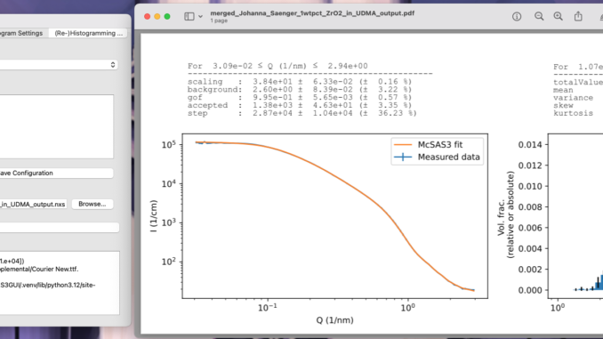
A few years back, I refactored the McSAS analysis software to enable multicore processing and re-histogramming, amongst other improvements.

As McSAS3 was command-line only (so that it could be easier integrated into data workflows), the uptake of that software has been rather low. So it was time to write a user interface for this, to help apply it to our data. This UI is now almost usable, so here’s a preview of what that looks like and what it will be able to do for you:

Differences from the OG McSAS

As the working concept of McSAS3 is drastically different from the original McSAS, it needed a different approach. First and foremost, McSAS3 is intentionally strictly separated from its user interface, as I want you to be able to run McSAS3 headlessly, in the background, as part of your data processing workflow. That means you could use it on a beamline, for example, for near-live processing of incoming data.

It’s all in the configuration files..

A consequence of that choice is that McSAS3 needs to be provided with configuration files. These are YAML files that tell it:

1. how to read in your data, be it in csv, pdh, or a flavour of NeXus. Also, what q limits to apply to this data, optionally step over any areas with peaks, and how many bins to rebin this data into. You don’t want too many bins for speed and sanity reasons, 100 usually will suffice.
2. how to run the Monte Carlo optimization, i.e. what model to use (from the SasModels library), what parameter limits to assume, and what convergence criterion to try and achieve. Since this convergence criterion is highly dependent on the quality of your uncertainties – by no means a given -, I also added the additional constraint of optimizing to a maximum number of accepted moves. 1000 seems to suffice for a reasonable fit
3. how to histogram or rehistogram the result. If you want your histogram settings different, you don’t need to redo the optimization itself. You just re-analyse the set in a different way. The histogram settings configure how many histograms you want, and what parameter ranges they should span. Population statistics are then calculated as well for that range.

The Data Settings tab

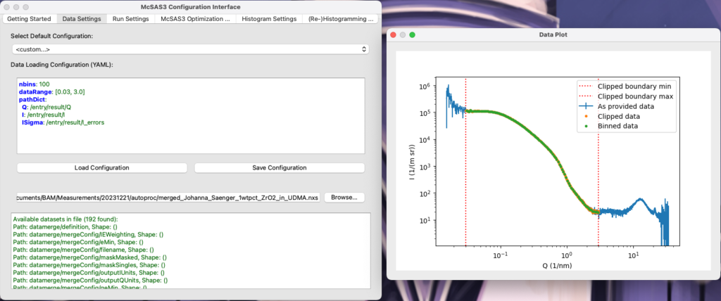
While this works, writing YAML files is nobody’s favourite activity. So the UI has three tabs to help you configure each of the above. Take, for example, the data loading tab. Here, you can first select a YAML example template and a test datafile, and then you can start editing the settings in the integrated YAML editing widget. When there is a brief lull in the writing, and the configuration is good enough to read the data, the UI will pop up a second window showing you the full data, the clipped data (i.e. data within the dataRange and with optional omitRanges stepped over), and the rebinned data that will be used for the optimization itself. It will update live when you change the settings. Once happy, you can then save your configuration and move on to the next tab…

The Run Settings tab

The run settings tab implements pretty much the same strategy as the data load tab. It has a few presets you can choose from, and then you can edit the YAML file. If you type any acceptable SasModels string (see the examples in the SasModelsExplorer blog post), it will list the available parameters. You can then choose one to fit, and either set a parameter value range (e.g. “[3.1, 300]”), or set it to “auto” which uses the radius* limits according to the q limits. Other, static parameters can be set in the staticParameters tab if they deviate from the defaults. A scaling and background optimization is automatically implemented as part of the Monte Carlo procedure, and so should not be defined in the staticParameters. Once you think you have a workable solution, click “test” and see if you’re getting anywhere.

A word of warning: McSAS3GUI does not have any guardrails installed. If you set the maxIter or maxAccept parameter too high, or the convergence criterion too low, that single optimisation might take a looong time. An “abort” method is in the works, but an elegant and reliable code segment has not yet been found to do this. So tread carefully.

The McSAS3 Optimization… tab

Moving on to the McSAS3 Optimization tab, this is where you can run the real optimization. Load your (list of) datafiles here, as well as your read configuration and run configuration (the latter two support drag-and-drop as well), and click “Run McSAS3 Optimization…”. Go for a coffee as the files are fit one-by-one. The repetitions of each optimization are spread over the available cores, so things might get toasty here. Optimizations all done, time to move to the analysis of the results!

The Histogram Settings tab

Now that you have successfully obtained sets of parameters that can fit your data, it’s time to move on to the analysis of said results. Histogramming the parameters is normally the way to do this. The Histogram Settings tab is again like the other two Settings tabs, with much the same functionality. Clicking “Test Histogramming” will execute that histogramming on the loaded McSAS3 results file, and open the PDF that it generates (sorry, this one’s not dynamically updating, but requires a click and a wait).

The histogramming section allows you to specify more than one histogramming range, which can be useful if you’re trying to pick apart multiple populations. These can be separated by a single line with “—” in it, which is the YAML way of indicating there are multiple entries in the one file. A second note: while it looks like you can show the results in different weightings than volume-weighted histograms, these are not implemented. Also, the minimum visibility limit famous from OG McSAS is not implemented either.

Of note is that these are not particle size probability functions, but particle size histograms. If your data was in absolute units, and the scattering length density correctly set in the model, the height of the bar is the total volume fraction of particles enveloped by the limits of the histogram bar. Similar, but not the same as particle size probability functions.

Once you’re happy with the way this looks, save the configuration and, if necessary, move on to the last tab..

The (Re-)Histogramming tab

If you have more than one file to histogram, this is the place where you can let your histogramming configuration loose on the stack of result files you have. It should be almost self-explanatory in the way it should be used.

So where are we at?

The code is functional, but not bug-free nor will it save you from yourself. It also has some minor installation issues: besides downloading the McSAS3GUI repository, you will need to symlink mcsas3_cli_histogrammer.py and mcsas3_cli_runner.py from the McSAS3 “refactoring” branch. into the root directory of McSAS3GUI. As such, it’s not yet recommended for users, but only for people familiar with python. Launching the UI can be done from the McSAS3GUI directory by typing “python src/main.py” (another indication that this is very much alpha release).

So now that 90% of the work is done, we can start spending ten times more time to get the final 10% of usability. So the v1.0 release may still be a while out, but at least you know it’s coming. If you leave positive feedback of my work at my bosses, and tell them how much you need this, they might even be able to assign some “resources”, as we are so inhumanely called, to free up some more time for me to work on this a bit more and get it done faster.

Until then, every help is appreciated, and help with the code is always welcome. We need unit tests, a better package name, an installer, an abort function, perhaps compilation of the code and its dependencies, a better way to call McSAS3 instead of symlinking, units support (mostly by improving the McData class in McSAS3, which I’m having to stop myself from refactoring altogether), and many updates to the guardrails, graphics and documentation.

Wish me luck.

*) I’d prefer using diameter, as per the recommendations in our data analysis round robin, but sasmodels demands I specify radii..