

Last week we spent a few days not measuring samples, but instead doing a few maintenance tasks that have been looming for a while. Let’s go over the improvements.
1. Power to the people
One thing that always irked me about the instrument was that it was fed from a single group (16A fuse). When we did experiments that required a lot of extra hardware such as heaters or chillers, that brought us rather close to the limits. Tripping a fuse or the RCD would mean potential damage to the X-ray sources, and cause lots of issues with our forgetful motor stages not remembering their positions (indeed, this is what kicked off the whole upgrade end of last year). So, time to tidy this up.
With the help of Anja as well as Sergej; a lab technician who joined us from another group, we quickly sketched the new power supply plan. The house electricians spent two hours rewiring the groups, and we now have a fancy division, spreading the load over seven (!) groups, three power lines and three RCDs. It’s overkill for sure, but this has us on a very safe margin for a while to come. The groups are now roughly divided into:
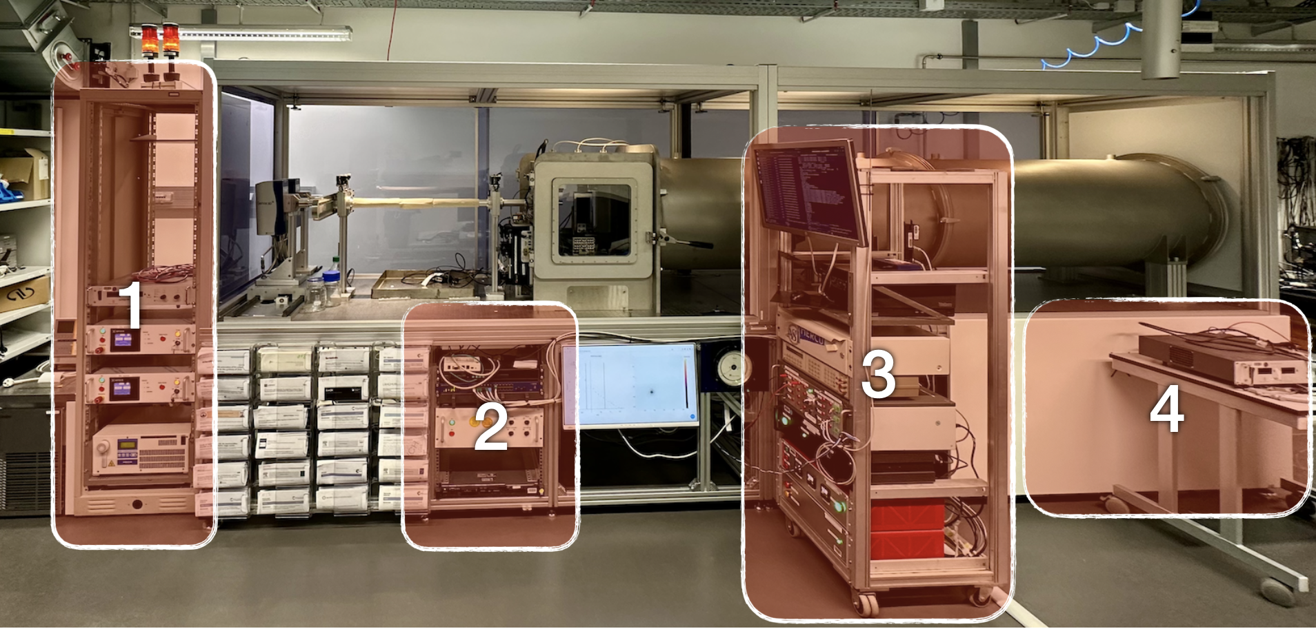
- The left-most 19″ rack, with X-ray power supplies / controllers and the source chiller.
- The machine rack; powering some small items such as the safety interlock, the motor controllers, the machine network switch and serial server, and the Dectris (detector) control computer.
- The control rack; containing the sample motor controllers, the control server and the Arduino Pro PMC general-purpose I/O box.
- The right side of the instrument, containing the detector chiller, the detector power, and the pirani gauge power.
Then there’s some extras, each directly powered by their own socket/group
- The high-capacity, Roots vacuum pump on a three-phase power supply, with its own 32A fuse.
- The chiller for that vacuum pump
- And lastly, all experimental power comes from a completely separate group with a separate RCD, this can be used to power heaters, chillers, and whatever else the users may want to plug in. If this trips, I will not shed a tear.
Groups 1-2, 3-6, and 7 are on separate RCDs. Also, every group only has one power strip connected, so no more daisy chaining and a nice clean power wiring set-up is the result.
2. Zeroing the slit blades (step 1)
As mentioned before, Anja implemented a method for her grazing incidence experimentation to shape the beam to her needs. Instead of manually aligning the 12 slit blades to produce “something that looks about right”, which is an inherently irreproducible procedure, she turned to Gaussian processes.
There will be more written on this in the near future (as it’s turned out to be more complex than I initially thought), but the long and short of it is that we can define our desired beam, and the Gaussian processes optimise the slit blade positions to get as close as possible to our wishes. So for our standard collimation settings, we used this method to optimise the slit positions to get a good beam.
The only problem with this was that we had not defined the slit positions to each other, and so had no idea what the actual slit positions and gaps were. We just know (and store) what the beam shape looks like on the detector, and we know the flux. This was enough during the hectic time at the end of last year, and we could continue measuring.
Fast forward a month or so, and we realise it is actually a good idea to have an idea about slit positions and gaps, and not blindly trust the automated processes. So this instrument downtime was a good moment to zero the slits to a common position, and simultaneously redefine the direction of movement for the slit blades so that their sign matches the external coordinate system.
For the zeroing, we started from our longest configuration, i.e. with the longest sample to detector distance and therefore the smallest beam. We then scanned each slit blade separately inwards, and by applying a linear fit to the region of 

3. Ophyd experimentation (zeroing step 2)
Knowing the zero position and direction sign is one thing, applying it is another. While for one or two motors this can be done by hand with a clear mind, for 12 motors we were bound to make a mistake. So we turned to scripting.
As our eventual goal is implementing the bluesky project ecosystem, a process we started by moving to EPICS control for the basic hardware control, we also have to get familiar with the ophyd hardware abstraction layer. This is a small pythonic layer on top of epics that groups the EPICS process variables into device classes. The extra metadata that thus emerges from the structure makes it easier later for the experimenters and the bluesky run engine to intelligently deal with the physical objects during an experiment.
With EPICS in place, ophyd becomes but a small, minimal piece of code. For example, I can now combine my four slit blades into one slit class, and add the pseudo-coordinates as well. With that, I mean I don’t just have the positions of each slit blade pair, but also can represent them as a blade pair defined by a “gap size” and a “position”. Translation is done transparently between these pseudo and real coordinates, making it easier for us to use. The ophyd abstraction for our detector is a little more involved, but that’s a story for another time (as soon as I have it fully figured out, that is).
Anyway, with each set of four slit motors now easily accessible via their ophyd abstractions, we could use the previously determined zero positions and directions to actually zero the drives, and to apply all the new offsets and sign changes to our previously determined configuration files as well.
Next steps…
So now the machine is back up, we checked all configurations with the newly zeroed drives, and the collimations look good. The beamstop seems to have misaligned a little as a result of the power down (that is a thing that happens), but by using the same Gaussian processes, the beamstop is easily realigned again for the configurations.
Next up is making the ophyd abstraction of the detector work well, and then we can start using the bluesky run engine to do a wider variety of scans and optimizations. It’s slow progress with this transition, but we are working on it in between measurements and experiments, time permitting. As always, I will keep you informed!