Correcting for transmission/absorption part 2… trouble ahead

Following this story on determining the correct X-ray transmission/absorption, I had to try and implement a solution. A pragmatic solution has now been implemented, and it appears to highlight three important points:

A decent method can be implemented to do proper transmission correction valid at different sample-detector distances, also compensating somewhat for the scattered and diffracted intensity.
With this method, we now also have a rough (under-)estimate of the scattering probability. Given the values we see in practice, we may be affected by multiple scattering more than we previously assumed,
if we don’t account for the scattered and diffracted photons, the transmission/absorption factors will be significantly off for many of the samples that cross our bench (exceeding several percent, sometimes even more than 10%). This will also affect the apparent thickness for samples where we use the X-ray absorption coefficient to estimate thickness.

Since we’re investigating regular samples, these findings could affect our entire community. So, let’s talk about it, and highlight some things I encountered along the way…

For the sake of brevity, please read this story first if you aren’t familiar with it already: https://lookingatnothing.com/index.php/archives/4453

The key points are that

we define transmission as everything that is not absorbed (i.e. absorption as the complement of the true transmission: $\mathrm{Abs} = 1 - T_{true}$ ).
Therefore, we have to also take all scattered and diffracted photons into account when measuring the transmitted beam flux (“method 1” for determining transmission)
If we only use PIN diodes or beam center-proximate intensity to determine absorption (“method 2”), we could be significantly off in our estimation of $T_{true}$ .
Practically, we may only be able to collect a limited segment of all scattered and diffracted photons (“method 3”), depending on how close we can get our detector and the shadowing of scattered and diffracted photons by sample holders.

In the end, I implemented two variants of method 3, both of which give us different information.

The variant for consistent transmissions

First, we need a way of determining transmission factors that give us the same results for multiple sample-to-detector distances (s-d distance). We vary this distance anywhere from ~100 mm from our sample to ~2500 mm. To get the same result from our transmission calculation, i.e. independent of the distance and fraction of scattered photons, we can use a circular area around the beam center (the beam center itself is determined using a scikit-image-based method).

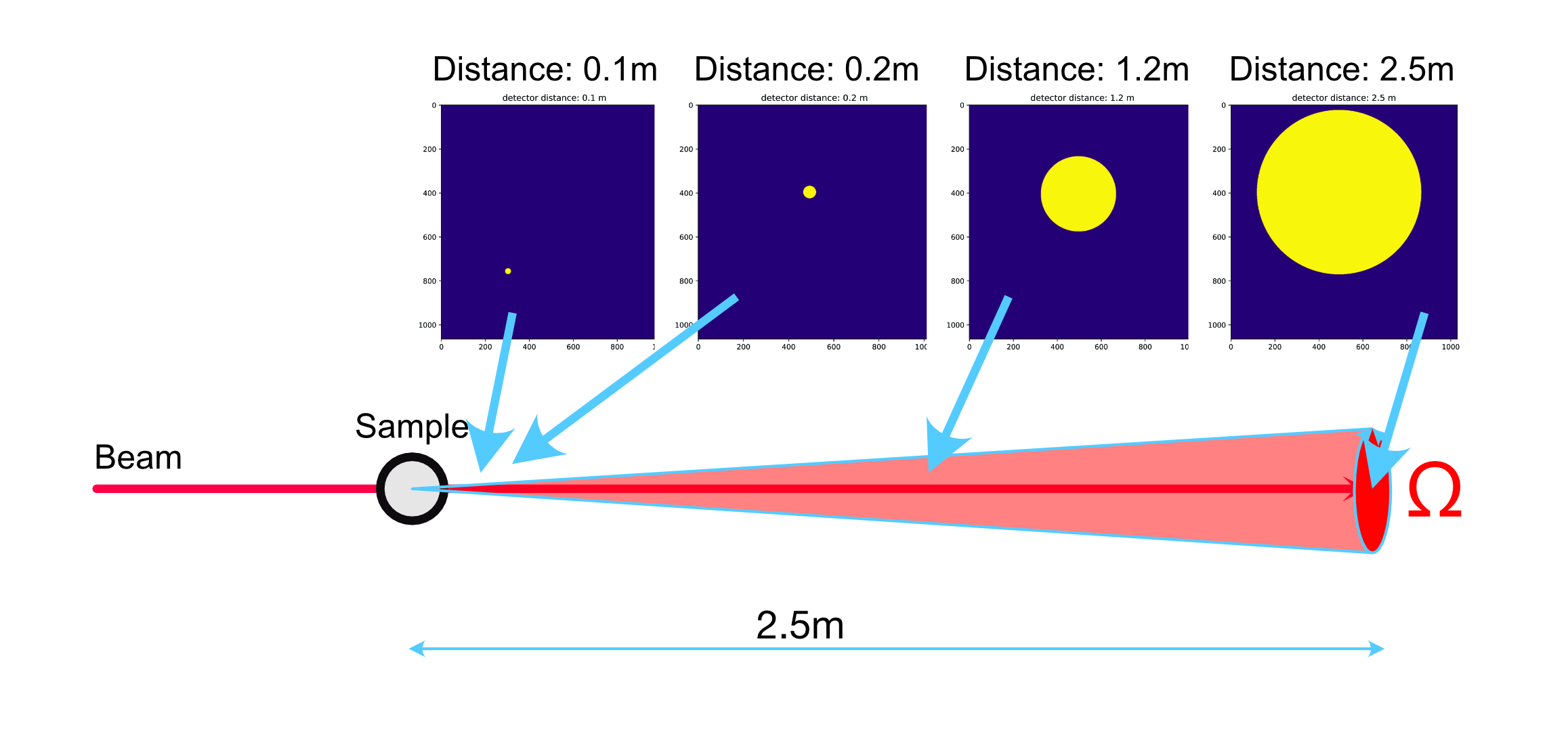
**Figure 0:** Beam masks over the detector area used at the various sample-to-detector distances to ensure a consistent solid angle coverage for the transmission factor calculations. Click to enlarge.

We set the diameter of this circular area proportional to the s-d distance, and use that mask to integrate the counts over the direct beam image (a), and the beam-through-sample image (b). If we choose a diameter of about 25-30 pixels at a s-d distance of 0.1 m, we have a large circle with a diameter of about 600 pixels just within the detector edges at s-d 2.5 m. These masks now are identical in solid angle, and so we capture the same scattered photons regardless of distance (this does ignore the finite beam size, but I assume it is not too significant given the area and beam sizes).

At the same time, we’re determining the transmission factor based on the whole image. At the closest distances (0.1m), comparing this image-based transmission with the beam transmission gives us a correction factor to compensate for the scattered and diffracted photons. The largest of these correction factors should then apply to all the measurements of that sample since the scattering probability does not change (but at larger s-d distances where our detector area subtends a smaller solid angle, we’re just detecting less of it). In practice, we do the following steps (see also Figure 1):

**Figure 1:** Flow-chart of the transmission determination process. Click to embiggen.

Scikit-image is used to isolate (“label”) the main feature in the direct beam image. This is filtered (to deal with isolated spikes and dead pixels) smoothened, and analysed to determine the weighted center of mass. This is our beam center.
We then determine a mask around that center, proportional to the s-d distance and a single diameter-distance combination. This mask is stored.
The mask is used in (a) and (b) to determine the primary $I_{0}$ and transmitted beam intensity $I_{t}$ . $I_0 / I_t$ is stored as the beam transmission factor $T_b$ .
The ratio of the intensity in the entire images $I_{0, I} / I_{t, I}$ is stored alongside as the image transmission factor $T_i$ .
A correction factor $c_f = T_i/T_b$ is also stored for every configuration.
The largest determined correction factor (for one of the six closest configurations) is propagated to the other images. This is pragmatically considered the closest to the true correction factor to calculate the true transmission factor via $T_{true}=T_b c_f$
$T_{true}$ is calculated for all configurations from $T_b$ with the propagated correction factor $c_f$
The correction pipeline is applied as normal with this corrected transmission factor $T_{true}$ .

With this process, we have a reasonable approximation for correcting the transmission factor for the scattered photons, while maintaining consistent transmission factors for the different s-d distances.

The variant for estimating scattering probability

We use a similar approach as above to get a rough estimate of the scattering probability for each sample. The scattering probability is the ratio of scattered photons to incident photons, without absorption (the scattering probability is related to the scattering cross section via a transformation as explained in this section of the wikipedia page on scattering cross-section). We can roughly estimate this by calculating the ratio between the total transmitted beam flux and the scattered photon flux at close distances.

Scikit-image is used to isolate (“label”) the main feature in the direct beam image. This is filtered (to deal with isolated spikes and dead pixels) smoothened, and finally fine-tuned so that the beam mask covers 99.7% of the total direct beam intensity (three sigma). This beam mask is stored.
in image (b) we determine the intensities of the beam under the mask ( $I_t$ ) and the total image intensity ( $I_{t,I}$ ).
We obtain a very rough estimate of the total scattering probability within the solid angle coverage subtended by the detector, by $P_s = (I_{t,I} - I_t) / I_{t,I}$ . Essentially, getting a value for the question: “how many of all the photons we detect have scattered beside the beam”. This scattering probability estimate is stored.

Since we’re only getting a beam mask that covers 99.7% of the beam, this means we’re always counting 0.3% too much in our scattering probability estimate. Conversely, since our detector only covers a modest portion of the unit sphere, we are missing a very large amount of scattering, and so are most likely underestimating the actual scattered photons.

A better method would be to calculate the scattering curve and extrapolate, and estimate the total scattered photons based on this extrapolation. Then this needs to be applied as a correction factor to the transmission, to redo the corrections with the new transmission factor (perhaps iteratively). Since it feels like this will be a lengthy process for a limited benefit, and as you will end up relying on extrapolations that make up data where you don’t have it, we’re not sold on implementing such a procedure at the moment.

The impact…

**Figure 2:** SRM3600 glassy carbon measured in our standard set of instrument configurations – without autoscaling anything. Overlap between the different ranges is satisfactory. Click to enlarge.

So.. after a few weeks of working with this, what did we find?

The new transmission corrections

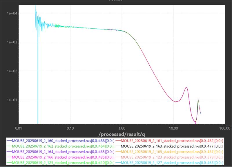
Let’s start with the good news. By virtue of $c_f$ , the SRM3600 curve is now 3.9% off of the published reference curve, a marked improvement from the 7.1% deviation with the previous method.

For homogeneous samples like glassy carbon, the scattering curves from the various instrument configurations also line up to a tee (Figure 2), highlighting that the absolute intensity calibration works well. We also took a measurement series with our molybdenum X-ray source, which also overlapped nicely with the copper curve, further underscoring our calibrations.

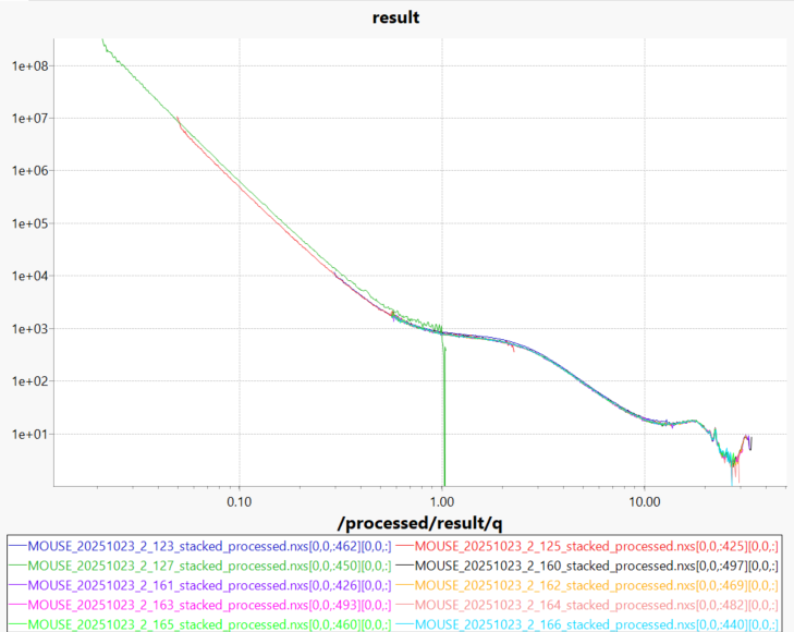
**Figure 3:** One of the worst offenders with the new transmission correction. What is going on with this sample?

For powders, however, the new method is not always the cure-all I was hoping for it to be. While the data from the different configurations for many samples now line up better than before, there still is the occasional sample where not every measurement lines up, for example the sample shown in Figure 3 (one sample out of a set of eight). I have double-checked the thickness and the transmission calculations, but can’t see anything obvious amiss. So, barring some programming mistake from my side, the alternative explanation is that this sample is not homogeneous. Then, by changing collimation, you’re illuminating different averages of sample. The investigations continue.

Until we find a satisfactory solution for this, we have no other option than to return to some autoscaling. Our autoscaling method is set up to automatically match the longer distances to the intensity of the shorter ones, can now do this sequentially as well, and stores this scaling factors alongside the data. See Figure 4 below for a preliminary investigation into these scaling factors of two months of measurements.

The scattering probability estimate

Since we now have an easy way of getting a rough estimate of the scattering probability as well, what do these look like?

As mentioned in the previous section, we will need to do an exploration over a larger cross-section of samples at a subsequent stage to get better insight into its prevalence. However, an initial inspection shows that a good number of samples in our instrument have a scattering probability that is on the order of several percent. This is not a worrisome number, as it indicates that the probability for double scattering is another two orders of magnitude lower, i.e. well below a percent. Double scattering here is used as a first-order estimation of all multiple scattering effects, as recommended by Adrian Rennie at one of the SAS conferences a while back.

There are a handful of samples, however, whose scattering probability exceeds 10%, some even hit 20%. Those samples are more problematic, and should be automatically flagged. With such scattering probabilities, the chance for double scattering are $0.01 \leq P_s^2 \leq 0.04$ , and so exceed our 1% threshold of significance. That is to say, they will affect the collected data by over 1% of the intensity. As it is a folding, or convolution of the scattering curve with itself, it affects the scattering curve in a non-uniform manner. Thus, the shape of the curve will change due to this phenomenon, which will be detrimental to the accuracy of the resulting sizing information (with the exact effect dependent on the shape of the scattering curve itself, annoyingly…).

On the distributions – impact on the last two months of measurements

The last months, we’ve been measuring mostly powder samples of carbon-based materials. We can use these as a preliminary reality check on the aforementioned scaling issues and the scattering probabilities.

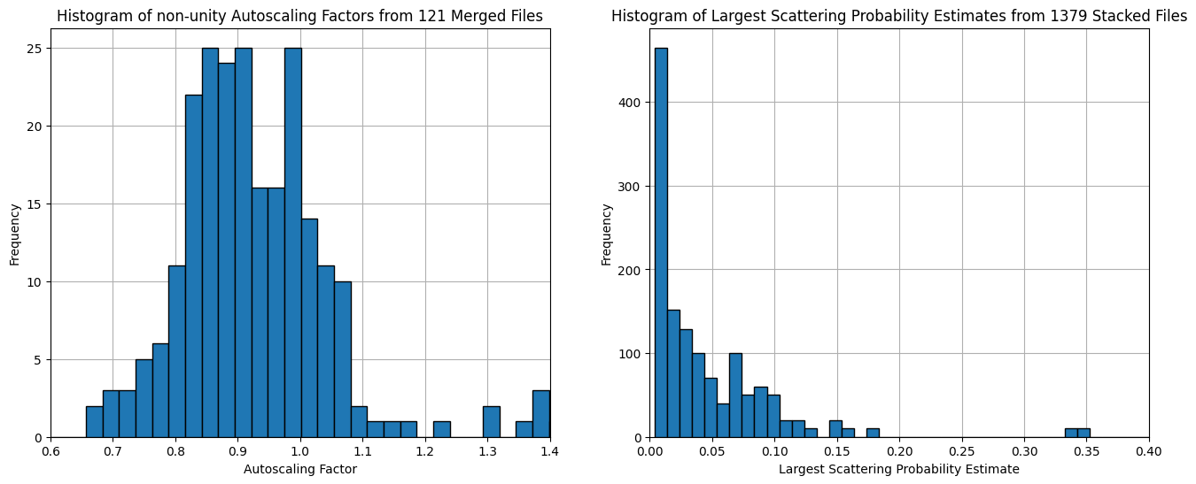
**Figure 4:** The scaling factors and scattering probability estimates over the last two months. Scaling factors between datasets of the same sample should be nominally 1, but are seen to vary by up to 20%, with a slight bias towards an effective intensity reduction. Scattering probabilities are seen to be mostly below 10% (which is good, this means double scattering probabilities are below 1%), with a small amount of sample scattering more strongly.

Figure 4 shows us the results of these, with the autoscaling factors determined for the longer configurations spanning the range from approx. 0.8 to 1.1. This is not ideal, as it highlights that for the powder samples we measure, the absolute intensity scaling is somewhat less precise than I am aiming for. This will need more careful investigation and probably will necessitate adjustments and compensations to better deal with the variability inherent in experimental powder samples. This might require more consistent sample packing methods, less freedom in the collimation settings, or other corrections not yet envisioned.

The scattering probability check, on the other hand, shows that we should be flagging a few samples for excessive scattering. The vast majority of the measured samples are fortunately in the green (i.e. with scattering probabilities below 10%), and so we can rest assured that the shape of the scattering curve is not likely to be significantly affected by multiple scattering effects.

Introducing flagging

As we are processing over 500 datasets every week (with typically 37 measurements for a single sample), the only way to help us find these issues is by introducing automated flagging to our data processing pipeline. These flags must then be brought to the foreground by an automatically generated report on the measurement series.

While we are doing some automated flagging (for fluctuating X-ray flux or unstable X-ray transmission factors), the flags discussed here for large autoscaling factors and large scattering probabilities have to be added as well. Subsequently, we have to think about report generation. As we are already assigning all our measurements to projects, it is not overly involved to program a reporting tool per project. These reports should show the datasets and a cursory initial analysis alongside other interesting information, but definitely have to put any raised flags first and foremost.

Conclusions and the next step…

So, all in all I am moderately happy with the new transmission factor calculations. The new distance-dependent masks make sure that the solid angle coverage is identical between the different instrument configurations and reduces the risk of inconsistent transmission factors. Furthermore, the transmission correction factor compensates somewhat for the elastically scattered photons, so that — even for strongly scattering samples — we are correcting only for the X-ray absorption. As we are also using that X-ray absorption to calculate the apparent sample thickness in the beam for powders, the thickness values should have improved a few percent as well.

While this story has become bigger than I had wished it to become, now that we have the information we seek, we should definitely exploit it. We will soon re-run the data corrections on all the measurements of 2025 with the current improvements, and report back on the more authoritative statistical prevalence of the aforementioned factors.

Looking At Nothing

A SA(X)S Weblog