

Since our revamp of the processes at the start of the year, we’ve been seeing a higher-than-normal variability in the absolute intensity scaling of the samples. Having since gone over and eliminated some potential causes in the preprocessing and processing pipelines, it is now time to investigate another potential source: the method with which we determine transmission factors.
How bad is it?
Initial check
To check whether we’re still okay, we recently measured the NIST SRM3600 glassy carbon standard for absolute intensity calibration. With our previous methods, our traceable absolute intensities were within 3% of the NIST reference curve (as determined using least-squares fitting of the scaling factor).
With the new method, however, this had increased to 7.1%. That means that for this particular sample, we are an additional 4% off. This could be a clue to solving our increased inter-sample variability if this difference can be traced back to sample scattering properties.
Does it matter?
We need to double-check whether any effort in this direction may be worth the accuracy gain, so a quick cost-benefit analysis is not out of place:
For our normal ~8.0 keV photons, glassy carbon scatters a reasonable amount: its scattering cross-section is on par with many powders we measure, and the powders usually scatter orders of magnitude more to smaller angles whereas glassy carbon flattens off there. Hence this would have a significant effect on data from realistic samples. Any offset in the absolute intensity would, furthermore, directly translate to a similar offset in any determined volume fraction and/or specific surface area. that means it is not only significant but it can also considerably impact final outcomes of scattering investigations. It seems worth investigating.
Possible cause
One difference between the previous and current implementation is the way we determine the transmission factor: the previous implementation simply integrated all counts over the detector area, regardless of sample-to-detector distance, whereas the new method integrates only over a square area +/- 25 pixels from the determined beam centre. Furthermore, we are using the transmission factor twice: once as a transmission factor, and the second time to determine the apparent material thickness in the beam (for powders and solids, at least, which has obvious issues for specific surface determination of porous samples, but we’ll get to that another time). That means the effect of the mismatch might be doubled.
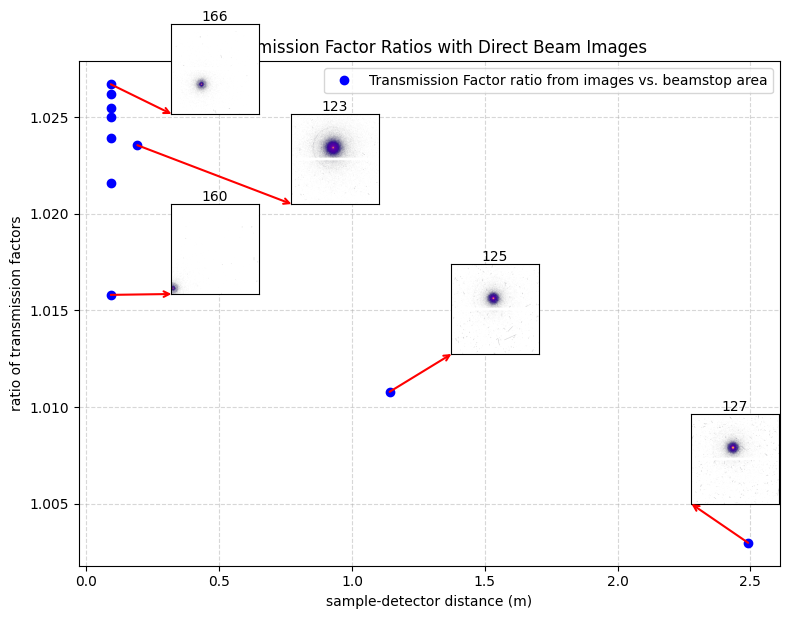
For our glassy carbon reference material, these two methods differ depending on the detector position (both dependent on lateral translation and sample-to-detector distance) as shown in Figure 1. As expected, we see that the difference is greatest (a bit more than 2.5%) when we capture more of the scattered intensity (the most for configuration 166: ~100 mm from the sample with the beam somewhat central), and least when we are far away (configuration 127 has the detector at almost 2.5m from the sample). So which is right?
The two definitions of transmission factor
The first way
In our lab, we always defined the transmission factor as the ratio of the photon flux of everything that has not been absorbed (and potentially re-emitted at lower energy), compared to the incident photon flux. This means that, to do this right, we need to measure 1) all of the flux that has not interacted with the sample, and 2) the total flux that has been elastically scattered. We’ll get to the practicalities of that in a minute.
The second way
The second way is more commonly used at synchrotrons, and mostly measures part 1). This is done by putting a (PIN-diode) detector inside the beamstop. That inherently means the transmission is determined based on the reduction of beam intensity in an extremely narrow angular range (sometimes not even covering the entire beam). Part 2) is then assumed to be orders of magnitude smaller and, therefore, not taken into account.
The third way
The third way is neither here nor there, and was the implementation used before: integrate over the entire detector. This approaches the first way when the detector is close, and approaches the second way when the detector is far.
We know the second way to be theoretically incorrect as well, as the transmission correction (at least in our correction pipelines) is supposed to be a correction for the reduction in interacting photons due to photon absorption by the sample. So the first way is the right way, but is hardest to implement.
So what should we be doing?
From practical experiments, we know that the overlap between our absolute-scaled curves measured in different instrument configurations is better when we use the second way for normalisation. That makes sense, as that gives more consistent results than adding an arbitrary amount of scattered photons. So the second way is the way to use for normalising measurements in different configurations, and is what we should do first. We may also want to consider integrating over different beam-proximate areas depending on sample-to-detector distance so the solid-angle coverage of the integrated region stays approximately constant.
We then should be correcting this transmission factor for the effect of the scattered photons. A pragmatic implementation would be to correct by the ratio between the whole detector area and the beam-proximate area for our closest, beam-centric image. Better would be if we would determine the total scattering information, and then integrate over the unit sphere as best we can.
For starters, we’ll try implementing the pragmatic way (second way, then the correction discussed in the previous paragraph), and I’ll let you know if that improves our precision and accuracy. The work continues…