Before I get started, let me just highlight the new small-angle scattering issue of J. Appl. Cryst. which has come out a few days ago. My contribution was unfortunately not accepted (and I haven’t worked much on it since due to rejection depression), but the journal is still very much worth a read!
Now for the main topic of today’s post. Regular readers will know that I have started implementing the “Everything SAXS”-set of data corrections in the Python language. Having worked on it in between other tasks (evident from the commits to the repository), it is now in such a state that it can do enough to do basic correction and reductions, with uncertainty propagation. At the moment, it is not very user-friendly (no GUI, for example), but it is modular and flexible, with an easy syntax. The correction modules are straightforward and easy to read and write, and Pythonistas will be able to dig right in and use it to do the necessary corrections. Here’s the details:The corrections implemented are (for the specifics, check out the paper):
- AU: for absolute intensity scaling
- BG: background subtraction
- DC: darkcurrent correction
- DS: data read-in and read-in corrections
- FL: Incident flux correction
- MK: Pixel masking
- SA: Self-absorption correction (plate-like samples only)
- TH: Thickness correction (important for absolute units)
- TI: Time normalisation
- TR: Transmission normalisation
- Integrator: An azimuthal integration module propagating statistics and calculating the standard error of the mean
Additional modules are available for:
- Calculating angles in various representaitons: Q and Psi, Qx and Qy, and Theta and Psi
- A 1D data writer (CSV files)
- A 2D data writer (HDF5 format, eventually to be NeXus and CanSAS2012-compatible) for storing intermediate datasets (background and calibration datasets, for example, which need to be corrected and used at a later stage)
- A PNG data writer (helpful for drawing masks in image editors on top of scattering images, for example)
- A 2D data reader for reading the background and calibration datafiles
Examples are included in the “tests” directory. There are two ways of setting the corrections: the most complex uses a “json”-file containing all correction parameters, their uncertainties and whatnots, allowing full tunability of the correction values. The second method uses a more direct keyword-value approach, but it only allows you to set the correction values for now (and not their uncertainties, though this will change soon to allow setting both). For today’s post, I will be demonstrating the second method.
Once you downloaded the correction software, the corrections can be done in a small Python script. I’ll first give the script for the background image correction, which you can gloss over but don’t have to understand. I will then explain what is happening using a second script for the sample corrections.
Here’s what’s done for the background correction:
import sys

sys.path.append('/Users/brian/Documents/NIMS_postdoc/python/imp2')

import imp2

imp2.DS(fnames = ['data/EmptyHolder_1_018.gfrm','data/EmptyHolder_1_019.gfrm',

'data/EmptyHolder_1_020.gfrm','data/EmptyHolder_1_021.gfrm'],

dtransform = 3)

imp2.FL(flux = 1.)

imp2.TI(time = 14400.)

imp2.TR(tfact = 1.)

imp2.TH(thick = 0.)

imp2.AU(cfact = 12.455)

imp2.MK(mfname = 'data/Bruker_mask_ud.png', mwindow = [0.99, 1.1])

imp2.QCalc(wlength = 12.398/5.41*1.e-10, clength = 1.052,

plength = [210.526e-6, 210.526e-6], beampos = [508.5, 533.2])

imp2.Integrator(nbin = 200, binscale = "logarithmic")

imp2.Write1D(filename = 'tmp/test1Dbgnd.csv')

imp2.parameters.writeConfig('tmp/bgndParam.impcfg')

imp2.Write2D(filename = 'tmp/bgnd2D.h5')

imp2.WritePNG(filename = 'tmp/bgnd.png', imscale = 'log')
There’s quite a lot going on there, right? Well, when this is run, it will nicely apply the necessary corrections to the background datafile (more specifically, to the four datafiles making up the background measurement). Now let me show you what exactly happens when we subsequently want to process the sample:
The first thing we do is just a bit of fluff for Python to load the data corrections:
import sys

sys.path.append('/Users/brian/Documents/NIMS_postdoc/python/imp2')

import imp2
Now we can get started on the data corrections, by loading a file. We want to load file Mehdi_Meng_1_005.gfrm (a Bruker image), and transform it a bit (flip upside down, if I’m not mistaken) to put it in the orientation we like. Each of these arguments comes in a keyword-value pair, in this case the keywords are “fname” for the filename, and “dtransform” for the data transformation:
imp2.DS(fname = 'data/Mehdi_Meng_1_005.gfrm', dtransform = 3)
I then want to normalise it to the X-ray flux of the generator. Since I don’t know this, I set it to 1:
imp2.FL(flux = 1.)
We normalise the sample intensity by time (21600 seconds):
imp2.TI(time = 21600.)
Correct for the intensity reduction due to transmission:
imp2.TR(tfact = 0.4)
Do the same for the thickness (actually, this is a placeholder thickness, for demonstration purposes only, as the sample wasn’t really 1mm thick):
imp2.TH(thick = 0.001)
We scale to absolute units using a separately determined calibration factor:
imp2.AU(cfact = 12.455)
Mask the image’s dead zones with a separately drawn mask (mask drawn in ImageJ on top of an exported raw detector image. You can use Photoshop as well, or any program you like):
imp2.MK(mfname = 'data/Bruker_mask_ud.png', mwindow = [0.99, 1.1])
We calculate the scattering angles based on the geometry (“wlength” = wavelength, “clength” = camera length, “plength” = detector pixel size, “beampos” = beam position in detector units):
imp2.QCalc(wlength = 12.398/5.41*1.e-10, clength = 1.052,

plength = [210.526e-6, 210.526e-6], beampos = [508.5, 533.2])
Correct for sample self-absorption:
imp2.SA(sac = 'plate')
Correct for the background with the datafile stored in the previous script:
imp2.BG(filename = "tmp/bgnd2D.h5")
Now we do some azimuthal integration into 200 linearly spaced bins:
imp2.Integrator(nbin = 200, binscale = "linear")
Write the 1D data to a csv file:
imp2.Write1D(filename = 'tmp/test1Dresults.csv')
Write the correction configuration for the books:
imp2.parameters.writeConfig('tmp/testParam.impcfg')
Write the 2D (unintegrated) image if we want to reintegrate:
imp2.Write2D(filename = 'tmp/2Doutput.h5')
Write a PNG file for taking a quick look at the corrected datafile:
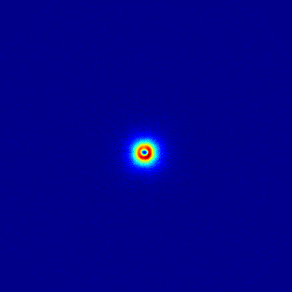
imp2.WritePNG(filename = 'tmp/fishies.png', imscale = 'log')

And that’s it for the basic corrections! So there are a lot of small steps, but each step has a clear and concise purpose and the associated values directly associated with it. The sequence of corrections is clear from the sequence in the steps, and can be rearranged if required. log-files are written and should be kept with the data for data provenance (a fancy way of saying that you can find out what you did half a year from now).
Still to do is to check the uncertainty propagation and to write the remaining correction modules. Some of these may take a while to write, depending on complexity. If you are interested in collaborating, help is always welcome (Git repository here)!

Leave a Reply