

One more burst of beamtime is coming up at the end of this week. This one will be with Zoë, Martin and Ashleigh once more, but there is one big difference: I ran out of funding, so I won’t be there!
Instead, for the first time, I will try to do a telepresence-kind of thing. I will be sitting here at my desk in Japan while the others toil away relentlessly filling capillaries at the beamline. My (self-appointed) task is “chief data-wrangler”: correcting the data and fitting it as best we can. So how are we preparing for beamtime (apart from loading and bringing about twice the samples you can ever measure)?
First of all, we had a good amount of e-mail exchanges with Andrew Smith from beamline I22. we talked about a host of things, including the set-up and many of the items mentioned in the SAXS measurement checklist (see appendix of this handy open-access review paper). This way, we can double-check the configuration and size-range we will be analyzing. Energies and calibrations have been discussed, and options for remote-access of files.
One more thing I started with a few weeks ago was to ask for some test datafiles. Each beamline (pretty much) uses their own data format, so in order to prevent unpleasant surprises I ask for a datafile in advance. I now set up the imp2 data correction methods to use this new format. The format used by I22 is one of the new formats, and one I very much would like to see adopted for “raw” data: the NeXus format.
This format is set up around a very flexible HDF5 data container, which allows for the structuring of data in a logical, hierarchical manner. This means that we can organise a complete set of information inside the datafile, such as motor positions, (multiple) images from multiple detectors, ion chamber read-outs, temperatures… Basically we can store everything that is relevant to the experiment and the data reduction. Let me show you what the structure of the data stored in this file looks like:┣━ entry1
┣━ I0
┃ ┣━ data: [ 1.26998004e+11]
┃ ┣━ description: [ ‘Data scaled by 1.0000e+06 and offset by 0.0000 for gain…
┃ ┣━ framesetsum: [ 1.26998004e+11]
┣━ It
┃ ┣━ data: [ 2.00207001e+12]
┃ ┣━ description: [ ‘Data scaled by 1.0000e+07 and offset by 0.0000 for gain…
┃ ┣━ framesetsum: [ 2.00207001e+12]
┣━ PilatusWAXS
┣━ Scalers
┃ ┣━ data: [Dataset array of shape (1, 1, 9)]
┣━ TfgTimes
┃ ┣━ data: [Dataset array of shape (1, 1, 8)]
┣━ detector
┣━ entry_identifier: [‘175549’]
┣━ experiment_identifier: [‘sm9612-1’]
┣━ instrument
┃ ┣━ PilatusWAXS
┃ ┃ ┣━ count_time: [ 10.]
┃ ┃ ┣━ sas_type: [‘WAXS’]
┃ ┃ ┣━ wait_time: [ 0.1]
┃ ┃ ┣━ x_pixel_size: [ 0.000172]
┃ ┃ ┣━ name: [‘PilatusWAXS’]
┃ ┃ ┣━ y_pixel_size: [ 0.000172]
┃ ┣━ Scalers
┃ ┃ ┣━ count_time: [ 10.]
┃ ┃ ┣━ description: [ ‘Timer (10 ns)\r\nQBPM (I0)\r\nIon Chamber (Not Insta…
┃ ┃ ┣━ name: [‘Scalers’]
┃ ┃ ┣━ sas_type: [‘CALIB’]
┃ ┃ ┣━ wait_time: [ 0.1]
┃ ┣━ TfgTimes
┃ ┃ ┣━ name: [‘TfgTimes’]
┃ ┃ ┣━ sas_type: [‘TIMES’]
┃ ┣━ detector
┃ ┃ ┣━ sas_type: [‘SAXS’]
┃ ┃ ┣━ wait_time: [ 0.1]
┃ ┃ ┣━ x_pixel_size: [ 0.000172]
┃ ┃ ┣━ y_pixel_size: [ 0.000172]
┃ ┃ ┣━ beam_center_x: [ 710.67]
┃ ┃ ┣━ beam_center_y: [ 78.33]
┃ ┃ ┣━ distance: [ 1.26401387]
┃ ┃ ┣━ name: [‘Pilatus2M’]
┃ ┃ ┣━ count_time: [ 10.]
┃ ┣━ insertion_device
┃ ┃ ┣━ gap: [ 6.08535]
┃ ┣━ monochromator
┃ ┃ ┣━ energy: [ 17.99999824]
┃ ┃ ┣━ energy_error: [ 0.002052]
┃ ┣━ name: [‘i22’]
┃ ┣━ source
┃ ┃ ┣━ current: [ 298.812]
┃ ┃ ┣━ name: [‘DLS’]
┃ ┃ ┣━ probe: [‘X-ray’]
┃ ┃ ┣━ type: [‘Synchrotron X-Ray Source’]
┣━ program_name: [‘GDA 8.38.0’]
┣━ sample
┃ ┣━ name: [[‘none’]]
┃ ┣━ thickness: [ 0.]
┣━ scan_command: [‘static readout’]
┣━ scan_dimensions: [1]
┣━ scan_identifier: [‘0712254c-0f97-4bc9-be55-0bb484dcd4b8’]
┣━ title: [‘Glassy carbon 18keV 1.2m 10s’]
┣━ user01
┃ ┣━ username: [‘GooglyBear’]
First of all, compared to previous data storage formats, this one is amazing. It is full of useful information and we can derive from the structure how the experiment was set up. There are some teething issues, though: there is a mish-mash of units used (and not specified), and all data is stored as an array for some reason. Information is power, though, and this format beats the pants off anything else out there.
There is also a lot of information in this structure we do not need right away, but is useful for future checks. This includes information on the insertion device motor positions and the synchrotron current.
Other information we do need. This includes information on the beam centre, the distance to the detector, pixel size and so on. I am now setting up the data correction methods to use these values.
There is some risk to relying on these values, however. For example, there is a value in the sample specification indicating the sample thickness. It is fine to have that there, but at the moment it requires input of the sample thickness by the user. Fail to set or update this, and you will be working with the wrong numbers. Beware, then, that the quality of the datafile (and subsequent processing) is reliant on the proper accounting dilligence for the values specified.
For this experiment, we will probably forego the “thickness” field anyway, and try to estimate it from the difference in absorption (also because the samples are dry powders). I will let you know if this can be done to any reasonable accuracy.
While progress has been booked – these data files can be read into the data reduction procedure, for example – , I am not quite ready yet. Before the beamtime, I must have a proper (semi-)automated manner for processing data in place and running. This will ensure that we can look at the data and analyse the data in place, and adjust the measurement procedure or samples accordingly. Time to get back to work!
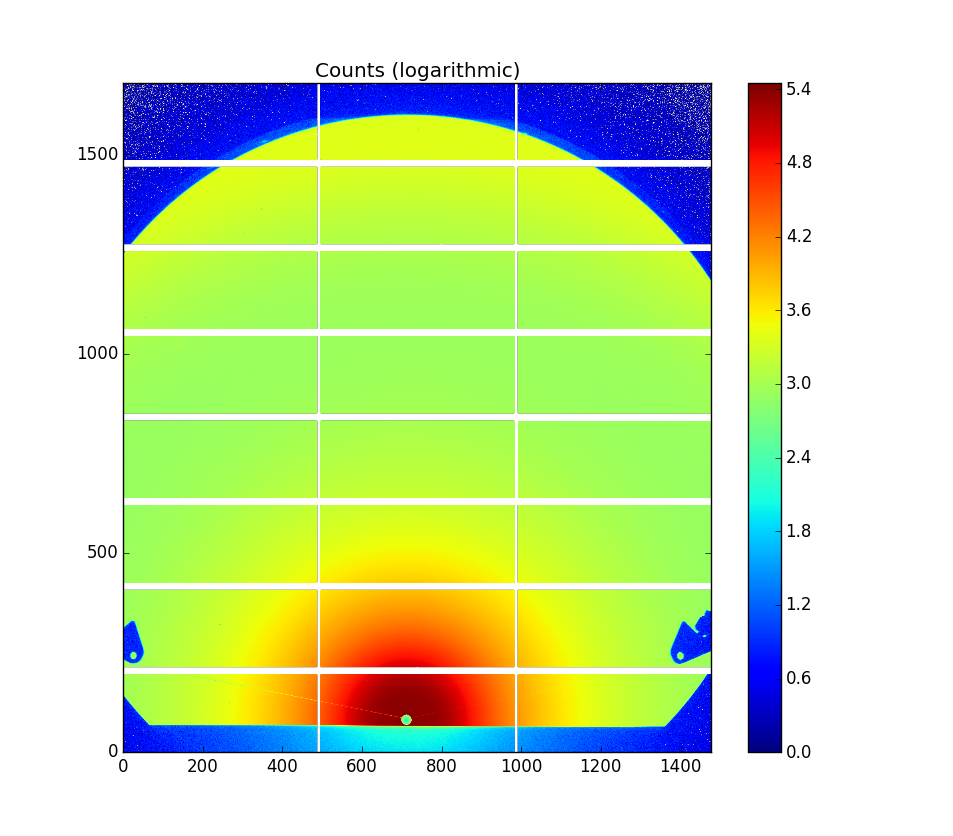
P.S. Look at how gorgeous GC looks on this beamline (Figure 0)!
(Many thanks to Andrew Smith of I22 for his rapid and helpful responses to my barrage of questions)
Dear Brian,
Regarding your article “Preparing for Beamtime” I find some things a bit bizarre.
You seem to be a prepared user, but honestly should the beamline not provide already a basic automated data reduction tool resulting in a fully corrected 1D scattering profile, so the user is able to focus on his data? This is pretty much standard today.
How would you be able otherwise to make full use of a SAXS beamtime at a 3rd generation synchrotron source?
HDF5 might be able to contain all your information, but what does it help if there is no data reduction tool in place that can handle those information?
It seems to overcomplicate things.
It is also not clear to me why the user would benefit from the information of the insertion device motor or the synchrotron current? Is there no transmission normalization in place?
There are programs like YAX, fit2d, pyFAI etc that should help you in case there is no automated data reduction pipeline in place. No need to reinvent the wheel if there are opensource programmes like pyFAI available.
Dear M. Bernard,
To answer one of your last questions first: the information on the insertion device gap and ring current is not immediately helpful (as we normalize by the incident flux monitor counts anyway, best monitored *after* collimation). However, this supplementary information can be very helpful in case you get results from your experiment that are inexplicable. Perhaps then you can trace that the (recorded) photon energy was not in accordance with the gap setting. Or maybe the ring current suddenly dropped for some measurements, meaning that these should be treated with caution (changing heat load on the monochromators can cause all kinds of funny shifts in experimental values).
As for the data corrections: I completely agree. The beamlines should provide the data in corrected and azimuthally binned format (for isotropic data) and corrected format for 2D data. This is the case already for many other techniques. When I asked about this at Diamond, however, the response was that their correction method is still in its early stages and isn’t ready for users (and not automated, and based on their DAWN framework which has a steep learning curve). So unfortunately it isn’t (yet) available from the beamline itself. They did make a good start, however, with the NeXus format containing (most of) the necessary metadata to do the corrections.
Furthermore, I am also full of (sometimes somewhat idealistic) wishes:
1) I want to have data corrections that propagate the uncertainty estimates through the correction steps. To my knowledge, very few programs take this into account.
2) I want to have a full suite of data corrections at my disposal, which I can then easily switch on or off. I covered the full suite in the “Everything SAXS” review paper on data corrections. While most of these corrections do not matter much for beamlines (where there is sufficient money for excellent new detectors), I also need to correct the data from my ageing laboratory instrument. This laboratory instrument occasionally needs some odd corrections, in particular a flatfield correction which can be determined through measurement of a glassy carbon calibration sample, but also darkcurrent corrections (despite it being a photon counting detector).
3) It needs to be possible to automate (because I am lazy and don’t want to manually process every datafile).
4) It needs to run on a Mac as that is what I use.
As for the packages you suggested: Fit2D and I never got along well in the past, it crashed too much for me and didn’t have a legible codebase. YAX I don’t know about but I will look into. To me, pyFAI (discussed on this site at the beginning of this year) is the biggest contender, and I have been following its development intimately. Let me spend a few more words on pyFAI.
pyFAI is designed to be (F)ast. This has major benefits at beamlines, but it also means the code is designed to be fast rather than clear: Jerome Kieffer explained to me that all the corrections are combined in just two image operations. However, this design choice also makes it more difficult to check the implementation and effect of individual corrections. As far as I understand, it also doesn’t propagate the uncertainties (yet).
What mostly stops me from using it, however, is that it does not run on my Mac. It is designed to be compiled and run on the (ESRF) Debian Linux release, using several optimization packages. Given the compiler shift on the Mac platform from GCC to Clang, some of the pyFAI-required packages don’t compile and the user interface is (therefore?) not working for me.
They do have a good team, and there is a good deal of activity on the GIT repository, so perhaps it will run eventually. If not I will just have to buy another computer to install their OS on.