Coherence in practice

During last week’s CanSAS meeting, I showed some new results on the coherence story. These appear to support the concepts raised earlier quite well.

To recap the general concern: the maximum size of objects that will scatter will generally be limited by the size of the regions in the sample where the radiation is in phase (coherent). The sizes of these coherence regions are typically much beyond the nano structural sizes probed by the SAXS instrument. However, for a sample with scatterers of a wide variety of sizes (such as some porous structures), we will still see the Porod scattering of the objects beyond the measurement range. It then follows that we should see more or less of this contribution added to our scattering pattern, depending on the size of the coherence volumes.

(Besides the size, there could also be a difference in degree of coherence. I.e. if the fraction of coherent vs. incoherent radiation is dependent on angle, the effect would be different than described above. In this case, we would see a direction-depedent scaling of the entire scattering pattern.)

The end result is that:

1. We will never be able to get comparable scattering patterns from disperse samples recorded on different instruments until we understand and correct for this. We will test if this is the case hopefully soon using the CanSAS round-robin method.
2. For instruments that exhibit angle-dependent coherence sizes (such as at synchrotron-based instruments), the scattering pattern will show anisotropy. This means that the simple azimuthal averaging procedure typically employed to obtain the 1D scattering pattern, will now average inherently dissimilar scattering patterns.

This latter point should be visible in our Diamond I22 measurements. If this is the case there, we should see a direction dependence of the otherwise rather completely corrected scattering patterns.

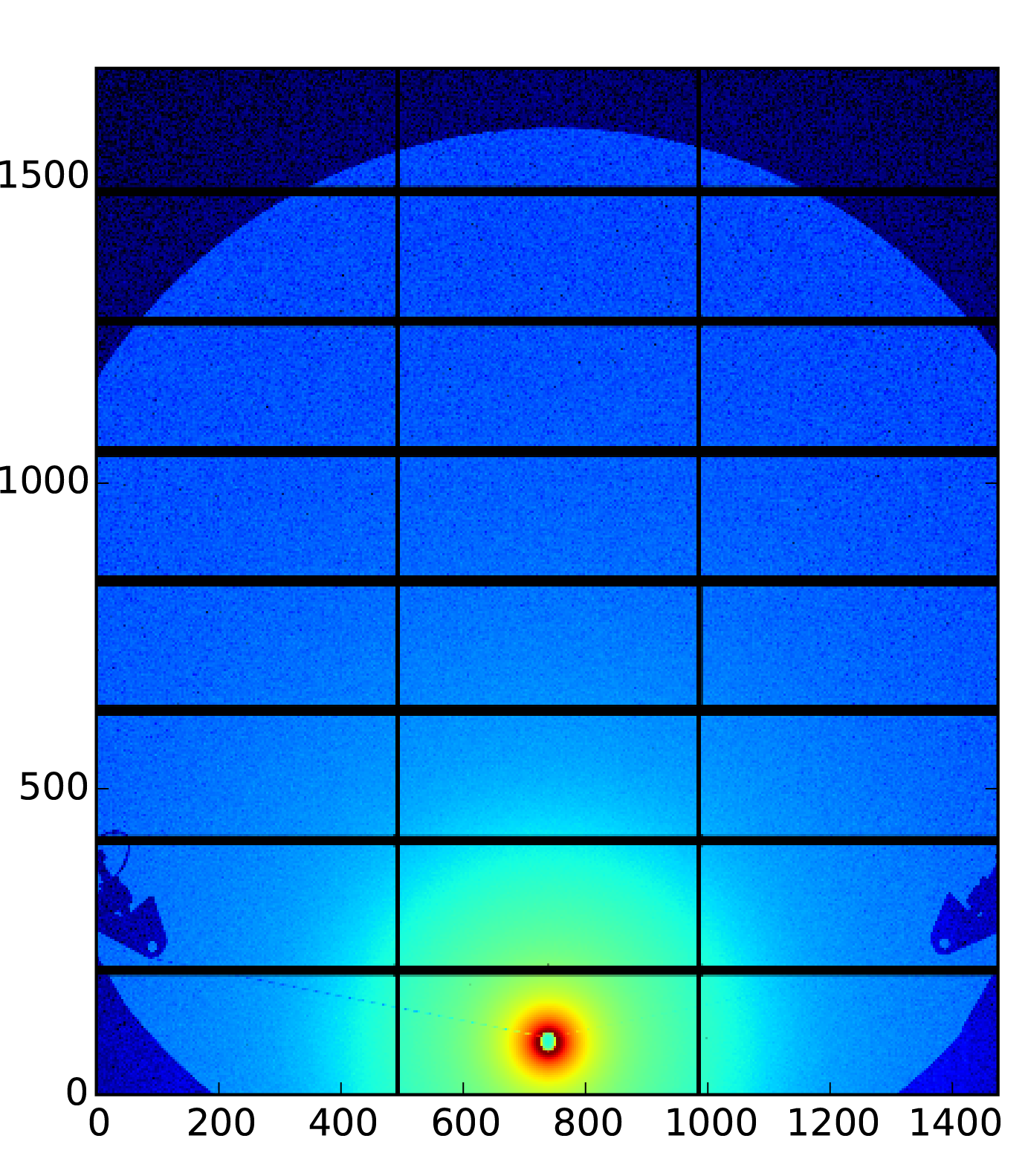
The original data is shown on logarithmic scale for one sample in Figure 1. Not much anisotropy is seen this way. When we apply the azimuthal averaging for this sample, however, restricting ourselves to angular ranges of 2˚ from vertical and horizontal, we do see a big difference (Figure 2). A line with a slope has been drawn as well. The difference between the two lines is about 32%, much larger than the vast majority of the corrections we are doing.

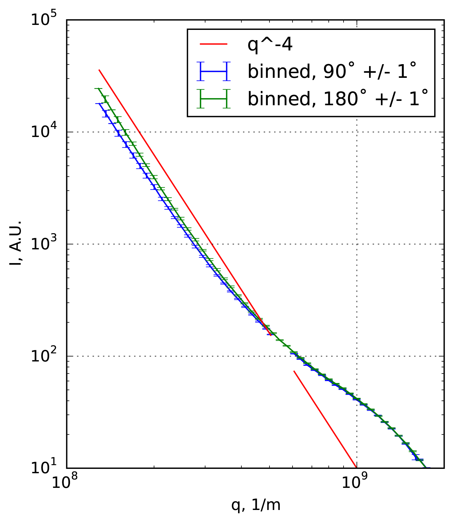
While the difference may be ascribed to preferential sample alignment, this is not very likely for powdered samples. Furthermore, similar differences are measured for five other samples (35%, 45%, 29%, 25%, 26%), and I do not expect us to be that good aligning dissimilar samples.

The direction of increased coherence, however, is opposite as to what we would intuitively consider correct. Andrew Smith of I22 has the following to say on that:

“I believe I have found an answer. S3 was the beam defining slit at 18.8m from the sample. This was set to 1 x 1 mm, which you might expect would give identical coherence in both directions. However, the beam shape at I22 is elliptical (with a profile of approximately 2.04mm x 1.28 mm H x V at S3)
So obviously we were constricting the beam to the more coherent central portion in both directions by not taking the full beam, but more so in the horizontal direction, leading to greater horizontal coherence. I think this makes a reasonably convincing argument.”

Taking this a little further, we can plot the relative difference of the patterns as a function of angle. For this, I have performed azimuthal averaging on 2˚ pie-sections for all angles between 1 and 181˚. We then plot the difference between these and the average of a 4˚ pie-section at 90˚. This is shown in Figure 3.

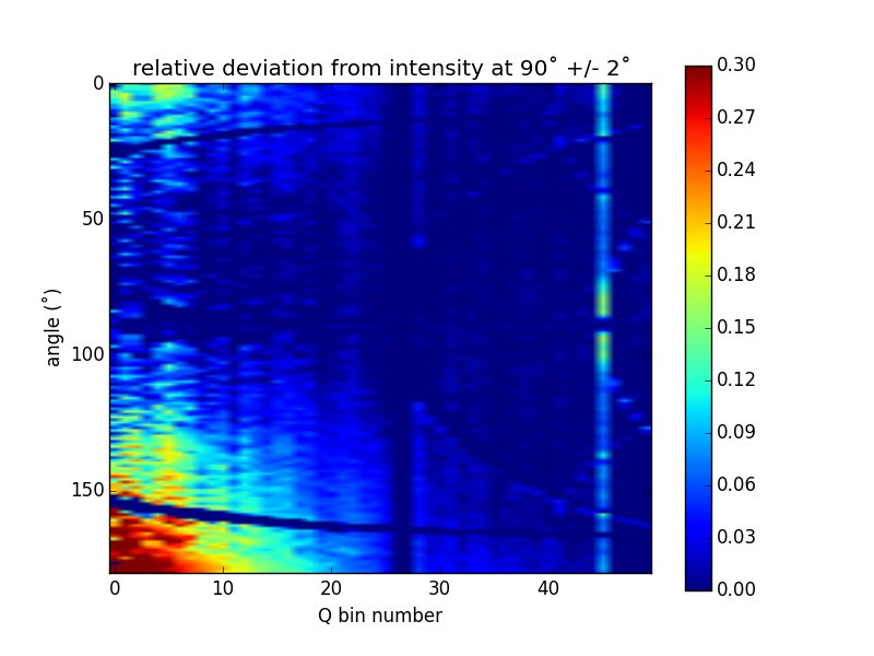
What we see is quite informative. We see that the anisotropy has a large relative effect in the first few bins, reducing towards the outer bins. This would be consistent with an increase in coherence size, but not with an increase in degree of coherence (i.e. the fraction of radiation that is coherent is independent of angle). However, the anisotropy axis appears to be deviating somewhat from 180˚, which may be inconsistent with the coherence story. (The curved lines starting at 30˚ and 150˚ are due to the shadowing of the beamstop wires, the vertical stripe at q bin number ~27 is a Pilatus module gap, and the edges of the modules appear to be slightly oversensitive.)

Performing this map for five samples, we see another interesting effect: the deviations are independent of the sample! It could be that we are effectively imaging the (reciprocal-space map of the) source coherence in this manner. However, such a conclusion has to be supported by someone more knowledgeable in coherence.

[ed: I removed this sentence when I realised that the minor fluctuations probably originate from uneven division of pixels close to the beamstop: “Moreover, the small fluctuations are also not changing per sample. These fluctuations look a bit like speckle patterns”]

If what we are seeing is due to the effect of coherence, its effect on the scatteirng pattern would appear to exceed that of all other corrections combined (save, perhaps, the background subtraction). By ignoring it, we are incorrectly averaging dissimilar patterns (and contributing unevenly over the q-range in the I22 case due to the offset beam centre location). Until such a time that a correction may be devised, the best course of action could be to limit azimuthal averaging to a certain azimuthal range.

We are now trying to get some more of this sample together for a round-robin test between instruments. The difference in configuration of the various instruments should highlight the differences in coherence between instruments. Furthermore, such a round-robin experiment may allow us to assess the degree of coherence in various places somewhat (though Yuya Shinohara assured me that a complete assessment of coherence in an instrument likely requires a bit more effort).

As usual, please leave your thoughts below!