

During the CanSAS meeting, a few comments pointed to the correct definition of transmission factor: “The ratio of the transmitted beam, plus the scattered and diffracted radiation, to the incident beam”.
For SAXS experiments (but not Ultra-SAXS), we usually smile at that italicized part and wave it off as a small effect. But we may get ourselves into trouble with strongly scattering samples…
Measuring a glassy carbon calibration sample should by now be a routine procedure in your toolkit. It is the one sample to keep close in times of metrological uncertainty. To measure glassy carbon correctly, however, one has to correct for the transmission: we need to compensate for the lack of detected radiation due to photon absorption in the sample. There are many ways of measuring the transmission factor of a sample 
According to the definition above, we can write:
With 


The definition above points to one good way of measuring transmission. If we are to place a large-aperture, high-dynamic range photon counter directly after the sample, we could measure both the photon flux of the direct beam as well as the intensity after the sample (
The next best thing would be a large area PIN-diode (I have some that are 10 
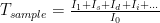
In our laboratory, however, we have a system that uses a sheet of 3mm thick glassy carbon (not calibrated) on an arm behind the sample (Figure 1). The idea then is that the scattering from that thick, strongly scattering sample is proportional to the intensity of the radiation impinging upon it. When the sample is not in place, the detected radiation is proportional to 


One common problem I may have raised before is that if you have a strongly scattering sample, this may pass through the 3mm thick glassy carbon (or, alternatively, cause a second scattering event in there). That means that in that case 

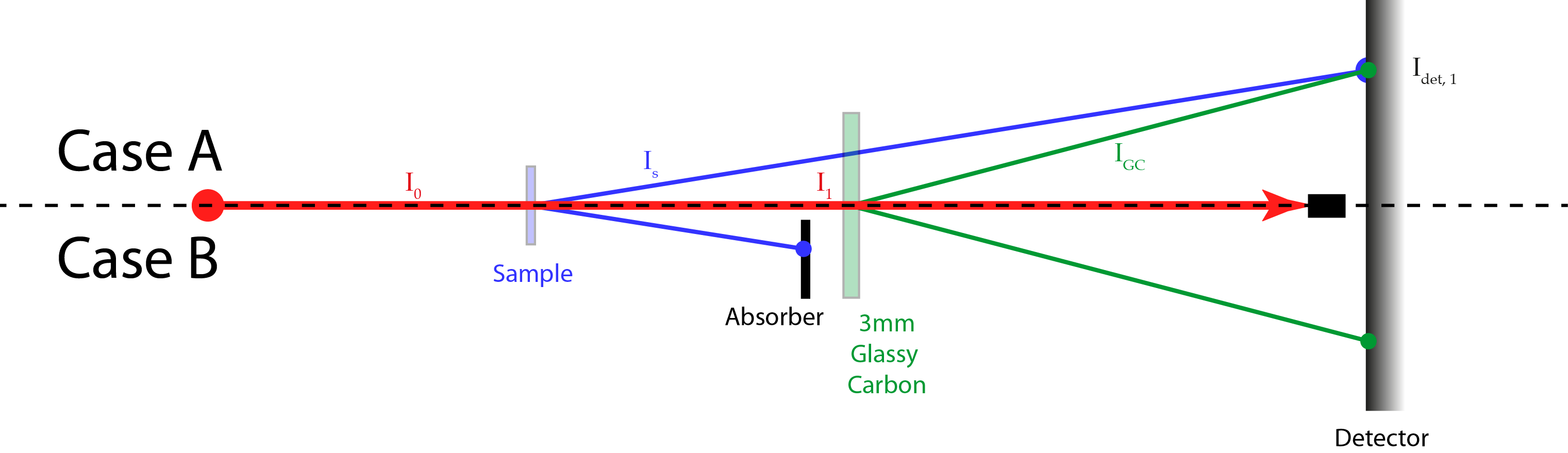
The easy solution for this is to install a collimator between the sample and glassy carbon, to prevent the sample scattering to impinge upon the glassy carbon or detector (Case B in Figure 1). This I have done long ago, and can be clearly seen in the transmission images obtained (Figure 2). We then use the counts recorded in the shadowed area only.
So what is the problem then?
The problem is our calibration sample. This calibration sample is a 1 mm piece of glassy carbon, whose scattering should be in accordance with a dataset measured on Jan Ilavsky’s instrument. Assuming a gravimetric density of 1.42 g/cc and a composition consisting of C, such a piece should give us a transmission factor of 0.955. Using our method, we get 0.90(1). Such a discrepancy I cannot accept.
It could well be that we are missing intensity in our transmitted beam
… and I thought I would have an answer for you by now. However, despite the simplicity of the posed question, I have yet to figure out how exactly this should be done. I am not even sure it can be done since we do not know the beam characteristics such as the degree of coherence. Hints and suggestions are welcome in the comments.
Hi Brian,
glad to learn you made it to Berlin, the city has a lot to offer. And sorry that I could not make it to the SAS conf, I had to stay at ID02.
The issue of scattering probability (which is far more common in SANS than in SAXS, with the additional issue of incoherent vs coherent scattering probability), is important and often neglected.
But evaluating it should in fact be rather trivial, as this is exactly what we measure on our detectors (assuming we cover adequately the q-range of interest), so we “simply” need to calculate the integral of the measured scattering intensity (only corrected by incoming flux, background, detector gain and quantum efficiency). We probably need to know the sample composition to determine the actual absorption, and atomic scattering which is not interesting for SAS. What bothers me is: (1) the measured “transmission” covers a solid angle beyond just the direct beam’s, so it also includes low q scattering, forward scattering (and null angle scattering, probably negligible) and (2) if there are two (+) populations of scatterers, is it correct to treat the whole q-range of data with one and the same scattering probability? For example, we are not interested in high angle scattering by atoms, these scattered radiations are as good as lost for us regarding small angle scattering. If you have large and small scatterers, should we not consider that radiation losses due to scattering by one of them should be removed from the flux used to correct the absolute intensity of the other?
I certainly need to sit and think quietly about these issues, which I find rather confusing.
But it is one of the reason I believe that the way forward in to complete data reduction (raw data to mostly corrected data) with data construction (best guess for data modified to reproduce at best the raw data), as many corrections are easy to add to a model, and not easy to remove from actual experimental measurements.
Hi Sylvain,
Sorry for the late reply.
You make good points as usual. The integration of the scattering curve on absolute scale should give us the number we are looking for. I think I should, however, integrate over the solid angle, not over Q as I tried to do when I did this investigation.
The issue with two populations is quite interesting, and may need to be clearly defined in publications that deal with these.
There was someone at the SAS conference working on complete simulation of the scattering systems, which would help us to sort these issues out. Hopefully we will see more on that later.