

Last year, I spent time (remote-) managing data corrections from Japan as the data came in at the Diamond I22 beamtime. Two more beamtime events are now upon us, same beamline, different samples. So what could be done to prepare for this?There are two beamtimes coming up, one starting this Wednesday until Saturday, and the other exactly one week later.The first will be in collaboration with Andrew Jackson, Duncan McGillivray, Nigel Kirby, Tim Ryan and Gloria Xun, who will be trying to put pressure on proteins. The second beamtime will be with Zoë Schnepp, Martin Hollamby, Ashleigh Danks and Dean Fletcher, doing some new, and hopefully elucidating, in-situ measurements on the cool category of ORR catalysts of Zoë’s group. Naturally, the stellar assistance from Andy Smith at I22 is indispensable in both of these.
The timing is a little unfortunate, as my workspace at home has been cleared out and put in boxes for the imminent move. Indeed, the second beamtime will be right in the middle of moving!
Nevertheless, there has been time to prepare, and with the generous aid of Diamond’s I22 Andrew Smith, tests could be run (on Diamond’s own systems using fresh measurement files) and the upcoming configurations discussed.
So by now you will go: “but you did all that before as well, what changed?”
Well, for one, the data corrections have become less convenient to use. Back then we had a more or less automated system, which would pick up the measurements from a directory, correct them and drop them in a “corrected” folder. However, despite the convenience, this could not distinguish between different types of measurements (background, mask, sample, calibration, etc.), and those needed to be manually done. Additionally, with automation comes risk: if things are not completely in order, by the time you will find out half of the measurements will need to be redone. I was completely beat after those two days of beamtime keeping everything in order.
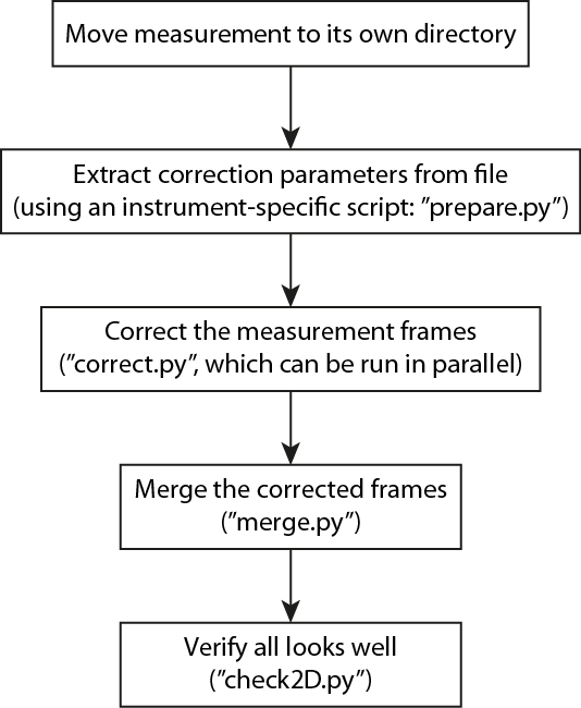
So this time there is a bit more interaction necessary to get things done, with added flexibility and time available to double-check before setting things off. The flowchart of actions is shown in Figure 1, naturally this can easily be scripted in a shell-script for more automation if so desired (eventually).
Now from this point in this blog-post, everything may become a little bit overly detailed. This is because this post also doubles as impromptu documentation. So if you are interested, read on (if nothing else, it will show you how much you can prepare for your beamtime)!
Let’s go over each step individually:
(1) Housekeeping
Moving (or copying) all the files belonging to a measurement to a separate directory is good for housekeeping. The correction program will generate a number of additional files (depending on the complexity of the measurement and the correction), which otherwise would just fill up your measurement directory unnecessarily.
If available, you also need to copy the background.h5 and mask.png files to that directory.
(2) Preparing parameters
Each instrument has its own way of storing relevant parameters. Some parameters, like monitor readouts may have values proportional to time, or not, and may need normalizing. Depending on the instrument configuration, other aspects need to be taken into account as well. This means that we need an instrument-specific script to extract and concatenate all necessary correction parameters, preparing them for the correction methods.
For Diamond I22, there is an additional complication, in that a single measurement file can contain multiple measurement “frames”, spanning two more dimensions. While theoretically everything is possible, I decided against implementing four-dimensional dataset processing in the imp2 correction methods. Multiple frames recorded on the same measurement location, however, is supported (and recommended).
So the “prepare.py” script prepares the correction parameters in a separate file. Based on your desires, it is possible to indicate that one or the other extra dimension is to be considered as multiple frames measured under the same measurement conditions (typically at the same sample position, as transmission and thickness correction parameters need to stay the same as well).
So for a Diamond measurement “i22-193140”, recorded with 10 frames (X) for each of 21 locations (Y) along the sample, we would want to do the f0llowing:
prepare.py --combineX i22-193140.nxs
This will prepare 21 files containing the parameters of the 21 positions. These files contain only a subset of all the information necessary for the corrections; immutable values are stored in a defaults-file.
If you are not measuring in different positions, i.e. you only have multiple frames, life becomes easy and fast:
prepare.py --combineX --combineY i22-193036.nxs
This will give you one parameters file. Careful, though for doing this for the 21×10 measurement: loading 210 detector images in memory will probably not work!
(3) Correcting
Now we are done with the preparations, we can get cracking on doing what we set out to do. Correcting the datafiles means indicating what the measurement was intended for: we need to select a correction pipeline (see this post on that). We do that for a single frame by:
correct.py -d ../defaults.json -p bgnd i22-193140_all_13.json
You see that the defaults are loaded with a -d option, the pipeline indicated with a -p option (available pipelines are “mask”, “bgnd”, “gcflatfield”, “gccal”, “sample” and “diamondsample”. Only “bgnd” and “diamondsample” are typically needed). Note that we are correcting based on a parameters file generated in the previous step.
This will correct that particular set of frames, and save the integrated data in a .csv file, and the corrected frames in an HDF5 (“.h5”)-file (with the pipeline tacked on to the filename).
To correct all 21 positions simultaneously, we encapsulate the “correct.py”-command in a for-loop (with a bit of shell script magic thrown in):
for i in `ls i22-193140_all_*.json` ; do bash -l -c "correct.py -d ../defaults.json -p bgnd $i &" ; done
When run in parallel like this, the whole process takes about a minute on my desktop Mac (4-core 3.4 GHz i7 iMac (late 2012)).
(4) Check
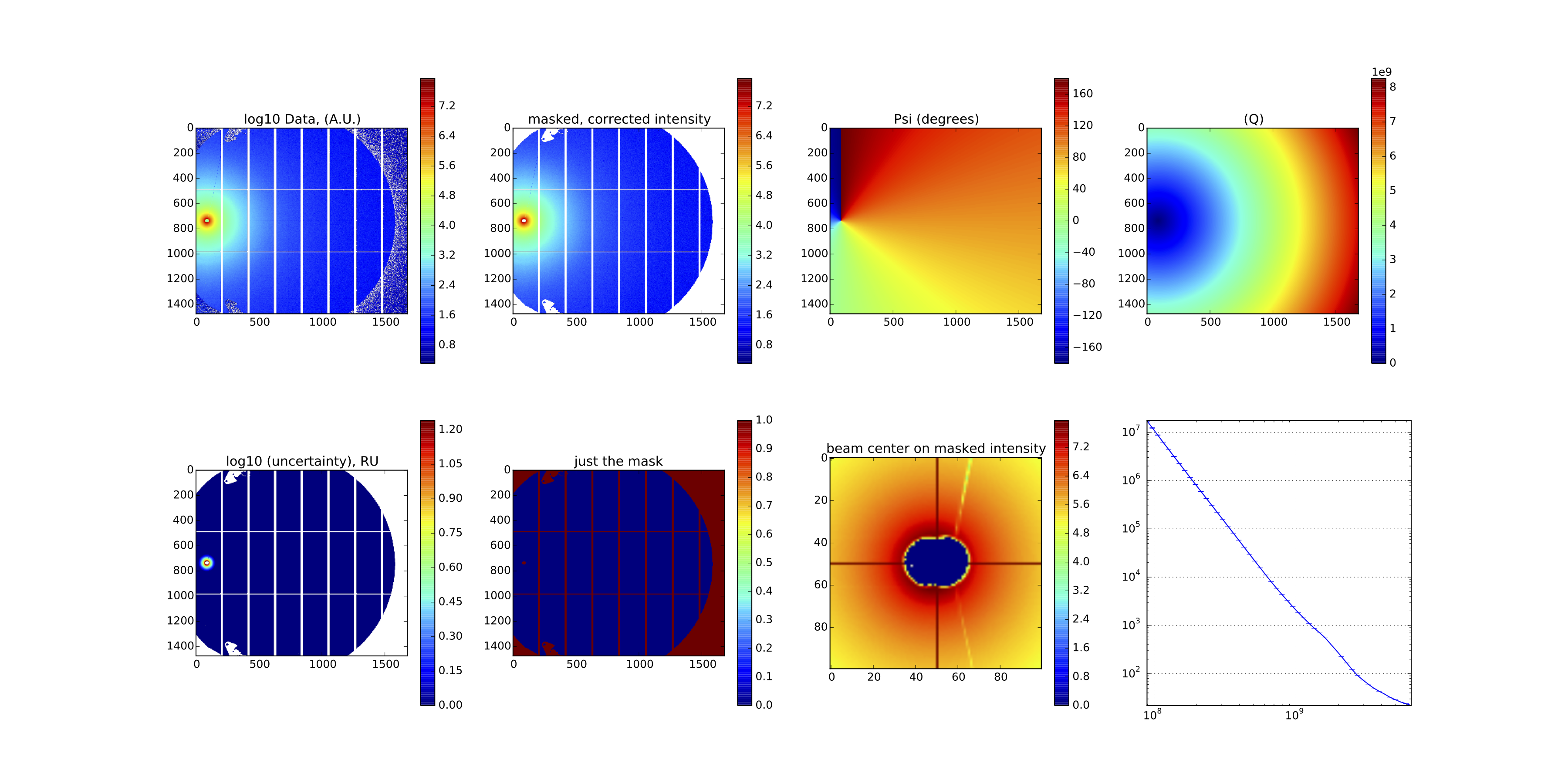
To check that the corrections went alright, a small (“dirty”) script has been prepared to produce a PDF file with most of the information we need. To run this on one of the HDF5 output files, we do:
check2d.py i22-193140_all_9_bgnd.h

Provided the script runs as it should, the resulting image should look like something shown in Figure 2. I admit, it doesn’t look like much, and that is a good thing: it is a background measurement of a borosilicate capillary!
Anyway, if this looks fine for a few measurements, continue on to the last step: merging frames.
(5) Merge
As indicated, we had measured this capillary on 21 positions along its axis, just so we could get a good average background measurement. Before we can use it as a background measurement, however, we need to merge the HDF5 files from the individual positions into a single background file.
That can be done using:
merge.py -o background i22-193140_all_*bgnd.h5
The options are almost self-explanatory (although for each program apart from the dirty “check2D”, help is available by saying “merge.py –help”). The last is the list of filenames to merge. The “-o background” indicates that we will save the result in the output file called “background.h5”. “-d” can be added but is a risky option, it deletes all the frames files once completed.
The resulting background.h5 file can be displayed again using the check2D script. Also, there is a h5Tree program in the imp2 tools, which allows you to check the contents of an HDF5 file:
imp2/tools/h5Tree.py background.h5
background.h5
┣━ imp
 ┣━ Qx: [Dataset array of shape (1475, 1679)]
 ┣━ QxRU: [Dataset array of shape (1475, 1679)]
 ┣━ Qy: [Dataset array of shape (1475, 1679)]
 ┣━ QyRU: [Dataset array of shape (1475, 1679)]
 ┣━ frames: [Dataset array of shape (1475, 1679, 21)]
 ┣━ intDataI: [Dataset array of shape (50,)]
 ┣━ intDataIRU: [Dataset array of shape (50,)]
 ┣━ intDataQ: [Dataset array of shape (50,)]
 ┣━ intDataQEdges: [Dataset array of shape (51,)]
 ┣━ intDataQRU: [Dataset array of shape (50,)]
 ┣━ mask: [Dataset array of shape (1475, 1679)]
 ┣━ workData: [Dataset array of shape (1475, 1679)]
 ┣━ workDataRU: [Dataset array of shape (1475, 1679)]
 ┣━ workDataSU: 783.429275685
┣━ sasentry01
 ┣━ sasdata01
 ┣━ sasdata02
And yes, that really is an attempt at a NeXus CanSAS link in there!
Processing a sample
A sample measurement works very similar to the method described above. In that case, however, copy mask.png and background.h5 files to the directory of the measurement, and proceed in a similar fashion. The pipeline in “correct.py” needs to be changed from “bgnd” to “diamondsample” (which is the “sample” pipeline minus the flatfield correction):
for i in `ls i22-193145_all_*.json` ; do bash -l -c "correct.py -d ../defaults.json -p diamondsample $i &" ; done
That diagnostics image (of the final, merged image) then looks like what is shown in Figure 3.
Sounds complicated…
Yes, it looks complicated, certainly more complicated than just copying the measurement files into a directory and letting the correction program plug away from there. However, the separation of steps and options to check hopefully makes life more easy when setting the corrections up. When everything is running, a script will be provided to to the sample measurements without many of these intermediate steps.
This blog post will update as the beamtime approaches with more information, perhaps with an easy meta-script for casual use.
However, my hope is that these efforts will make life easier for the people plugging away at the beamline. Doing measurements at the beamline is stressful enough as it is, and offloading the data correction can alleviate some of that stress.
Leave a Reply