

When correcting data for the many possible data artefacts, I usually prefer to do these corrections on the 2D images as opposed to the azimuthally averaged data (often referred to by the misnomer “integration”).
This needs to be done for some direction-dependent corrections, such as for the polarization correction, but not necessarily for others. The background correction, for example, can be done in two ways: subtracting the background image (2D) from the measurement image, or subtracting the azimuthally averaged background data (1D) from the azimuthally averaged measured image.
To illustrate the difference, perhaps a small demonstration can suffice.
Set-up
We define two images: a background image and a sample measurement image. These are completely made-up images, and we give them the nice property that they represent scattering images in polar format: only Q varies along one axis, and only the azimuthal angle along the other.
We imagine that there is a systematic instrumental contribution in the image: perhaps a small contribution from scattering off the edge of one of the slits or pinholes (streaking). Similar scattering can originate from capillary walls or imperfections in window material.
We create two images (Figure 1), 16 by 20 pixels in size, that represent the background and sample measurement. The background image contains zero counts with Poisson noise added, and 30 pixels with an elevated intensity. The sample image is set up in a similar way, with Poisson noise added, and 30 pixels of elevated intensity, but has 20 counts of “signal” added.
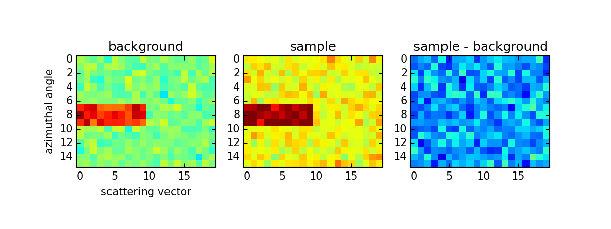
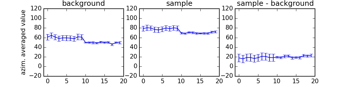
We can then attempt to retrieve the signal by subtraction of the background from the sample measurement in two ways: by subtracting the images followed by azimuthal averaging (Figure 1), or by azimuthal averaging followed by subtraction of the averaged data (Figure 2).
Conclusion
The conclusion is represented in Figure 3: both approaches result in the identical retrieval of 20 mean counts of signal after subtraction of the background. However, the region of elevated intensity results in a much higher uncertainty estimate on the data subtracted after azimuthal averaging. If we do image subtraction of the background before averaging, such spurious signals can — if they are stable in both measurements — leave no large detrimental effect.

@drheaddamage Just wondering what you use for error propagation? I got a good reminder yesterday that if one is trying to calculate a/b and both a and b have uncertainties then
 if you only use simple error propagation (i.e. one is ignoring the correlation).
Hello Andrew,
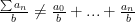
For the error propagation, I am assuming at the moment that the uncertainties are uncorrelated. In this case, the uncertainties should propagate for additions and subtractions as:

A correlation term can be added, but only if you have an estimator for the uncertainty on that correlation. There is a useful paper from NIST summarizing these here.
Not many people do error propagation yet, but I certainly hope that it will be in the near future. We could do with a better understanding of our data.