A few weeks ago, I posted a short story on the q uncertainty determination. This is now expanded, and based on the comment from Fred, it has been reworded to avoid confusion. In summary, it might be time to think about the uncertainty in our q-vector. The full story goes like this:

An assessment of the calibration of, and uncertainty in q

By Brian R. Pauw, BAM Federal Institute for Materials Science and Testing.

Introduction

The core determinant for the precision and accuracy in the established radii is the variation we might encounter in q. This encompasses the shift and scaling of the q-axis, the per-datapoint accuracy in position, as well as the spread of arriving photons in q. The latter is colloquially known as “smearing”, effecting a blurring, or smoothening of the scattering pattern. We will address each of these contributions.

The smearing

The smearing occurs due to uncertainties in the q value of a given detected photon. Over an ensemble of photons, this arrival position uncertainty distribution is typically centrosymmetric and ideally narrow. It leads to a reduction of definition (sharpness) in the detected pattern, similar to the “blurring” effect in image editing software, and is colloquially known as “smearing”. Analogous to the image editing example, the process can be partially reverted through an edge sharpening operation, in scattering parlance referred to as “desmearing”. This desmearing process, however, is mathematically challenging, magnifies uncertainties, and can introduce or miss features in the data.

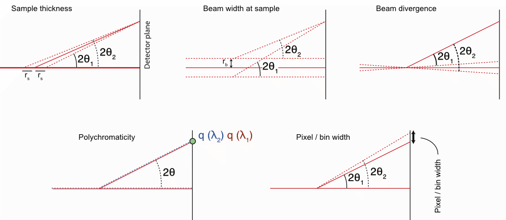
Smearing has a few causes, such as practical geometric limitations, wavelength dispersion, and detector imprecision (Figure 0). The centrosymmetric nature of the effect, and the optional desmearing step, however, can partically reduce the significane of the smearing effects. Nevertheless, it is always prudent to estimate the severity of the smearing contributions in order to provide a ballpark figure for the real uncertainty.

The per-datapoint position accuracy

One of the contributors to the smearing mentioned above is not just part of the smearing contribution, but also forms the lower limit of the uncertainty in q. Its fundament lies in the accumulation of photons with almost-but-not-quite-identical q values for a given datapoint. This per-datapoint position uncertainty is typically determined by the detector pixel size for raw data from pixel detectors, or bin size for binned data.

The scaling and shifting accuracies

For every instrument, practical limits on the knowledge of the instrument geometry leads to an uncertainty in the scaling and shift of the q axis. It is possible to estimate these two contributions practically using available calibration samples.

The plan

This document evaluates each of the three main effects in turn. We will first estimate the effects contributing to the smearing of our data. This section also contains the per-datapoint uncertainty that forms the minimum q uncertainty, which will therefore not be repeated. Secondly, we show our practical estimations for the scaling and shifting accuracy using a variety of calibration samples. Lastly, we will estimate the effect of these uncertainties on the size distribution parameters derived from a scattering pattern of silver nanoparticles.

The smearing

The geometry of the instrument

The Kratky camera employed for our measurements, has an approximate (fixed) sample-to-detector distance of 307 mm and a sample radius of 1 mm. The pixel size on the Dectris Mythen detector attached to our Kratky camera is 50 m, with no point-spread function. The X-ray spectrum reflected by the multilayer optics largely consists of Copper k and k radiation, whose mixture gives us an weighted apparent wavelength of 0.1542(2) nm. When we assume perpendicularity of the detector with the point of normal incidence at the beam center, the . The useful data in these experiments has been defined to start at .

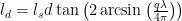
The finite sample thickness contribution

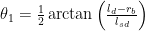
We can determine the sample thickness-induced uncertainty in q, , using:
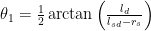
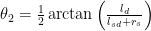
where
and

where is the distance on the detector from beam center to the point of interest.

We calculate from our reference q vector using:

The resultant ∆q due to the sample thickness: 0.0028

The finite beam height contribution

This is the issue of the beam not being infinitely thin. That means that scattering originates from multiple heights in the sample. This is calculated virtually identically to the above correction, except that we are adding the radius of the beam to instead of :

and

This results in a ∆q due to beam finite beam height of latex \mathrm{nm}^{-1}$.

The uncertainty originating from the beam divergence

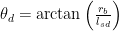
The beam divergence is dictated by the collimation as well as the optics. In our instrument, the beam is focused on the beamstop, and using that information together with the width of the beam at the sample position, allows us to estimate the effect of divergence. This calculation can be done quite similar to the estimates from before, but where we add the divergence angle from the straight beam to the angles:

and

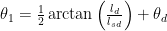
where

The total effect due to beam divergence adds (in the worst case) a ∆q of 0.185 .

The polychromaticity contribution

The emission lines passed through by the mirror contain both the as well as the energies (actually, the mirror also allows through higher order energies from brehmsstrahlung, but that is another problem for another time). These two energies bring about a small change in wavelength, and therefore q-vector. It is very small, but we include it here for completeness.

We estimate the thereby induced uncertainty in q, , using:
where

This calculation results in:

Copper ka1 wavelength: 1.5405e-10 m, Copper ka2 wavelength: 1.5444e-10 m
The relative uncertainty ∆q/q due to wavelength differences: 0.0025 .

The uncertainties originating from pixel or datapoint widths

The finite pixel or datapoint size gives us a width in q that can affect the resolution of the smaller scattering vectors.

We distinguish between pixels and datapoints, as the data in multiple pixels may have ended up in a single datapoint during the averaging or re-binning procedure. Geometrically, we have a lower limit of the precision defined by the pixel width. As given in the geometry section, this means that we have an uncertainty of no less than at , or 7 %. For the pixels higher up in q, this uncertainty will gradually decrease.

The minimum q-point distance in our example, binned dataset is the same at , implying that we have not lost precision through the re-binning procedure for the first datapoint. For the later datapoints, however, more and more pixels have been grouped together to form a single datapoint.

Along the q-vector of our measurement, the relative ∆q/q span of each datapoint can be determined as the distance between datapoints, and is approximately constant at 3.5 % of the q-value.

Smearing effect evaluation

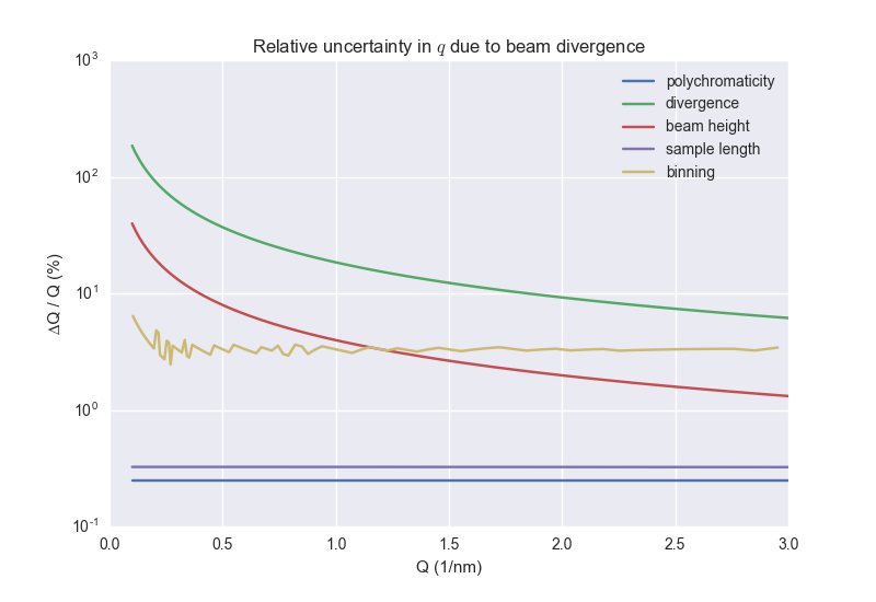
The relative contribution of each uncertainty contributor is shown in Figure 1. Here we see that the contributions of divergence and beam height contribute significantly, although these might be (partially) corrected for in our desmearing step.

The effect of the divergence on an example scattering pattern is shown in Figure 2.

Discussion

There is only one dominant uncertainty contributor to the smearing contribution, which is the divergence. As this contribution is significantly larger than the remaining contributors, the total uncertainty budget is accurately described by this sole contributor, and a calculation of the total uncertainty is not necessary.

The effect of the divergence can be shown on our example silver nanoparticle dataset in Figure 2, where it is a significant contribution. Indeed, it is so large that it raises questions about the validity of the estimation in practice. The effect in practice would be a broadening or smearing of the scattering pattern by a given divergence distribution function, the width of which is as described above.

We do have a plethora of arguments (excuses) ready on why it may not be as bad as this worst case scenario, for example 1) The beam convergence angle is weighted towards the horizontal, and so it isn’t all that bad… probably, or 2) We didn’t take into account the single-sided limitation to the divergence potentially introduced by the Kratky collimation.

The worst of the arguments (in terms of traceability) is that we perform the rather black art of desmearing on the data once received from the instrument. That means that some of the broadening in q has been counteracted at the penalty of higher uncertainties in the intensity. The thus-introduced reduction in our q uncertainty is very difficult to assess. We are therefore in this case limited to using practical estimators for the uncertainties, at least in the case of the Kratky-class instruments.

For an instrument based on a parallel beam, we could consider evaluation of the direct beam dimensions on the detector, which immediately encompasses three out of five of the considered effects. This is not possible in this case, as the focusing of the beam on the beamstop (close to the detector) “hides” the divergence effect.

Instead, we would like to use an evaluation sample which would show narrow diffraction lines on the detector such as tendons or optical gratings. These samples would allow evaluation of the broadening effects of the beam. However, these are not at hand for our slit-focused instrument.

Of note is the uncertainty introduced by the datapoint binning. This is not only a smearing contributor, but also the lower limit of the real uncertainty in q. Using the current binning scheme, it is a constant contribution at about 3.5% of the q value.

The scaling and shifting accuracies

The accuracy of the scaling and shift our q vector may be assessed using calibrators. These are:
1. Calibrant-based: Silver behenate, Apoferritin, Glassy Carbon
2. Geometrical considerations

The purpose of these calibrants is to determine the practical variance in q position for datapoints along the detector, and the shift of the entire q scale.

Evaluation of the effects of the uncertainties in q

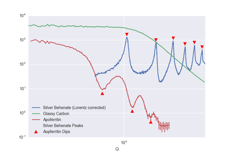
We measured silver behenate, Apoferritin and Glassy Carbon to practically assess the calibration and uncertainties of q (Figure 3).

Silver behenate is a commonly used sample for distance calibration, and is particularly convenient on the Kratky camera since it allows the assessment of a total of six peaks within the measurement range. Comparing the positions of the six peak maxima with the expected values allows the proving of two geometrical assumptions: the sample-to-detector distance, and the beam centre position. An offset in the beam centre will show up as a consistent divergence of the subsequent detected relfections with respect to their expected values. likewise, the determination of the maxima will give us not an accurate, but at least a workable estimate on the datapoint q variance.

One criticism of silver behenate as an absolute q calibrant is its instability: it can absorb water, thereby changing the crystal lattice somewhat. Some have indicated its components might also be degraded (affected) by light. An alternative calibrant, available in large quantities and of very well-defined shape is (equestrian) Apoferritin. This core-shell protein exhibits clear features in the scattering pattern and scatters well. Its fundamental pattern can be calculated using existing bead-model techniques, and modeled using a core-shell sphere function. We use this here to double-check our silver behenate calibration.

Glassy Carbon is not typically used for q calibration, being primarily intended for absolute intensity calibration. However, based on the initial results in the subsequent experiments, it may be possible to use this for both with reasonable accuracy. Its easy availability, high scattering, stability and solid state makes it ideally suitable for calibrating instruments without liquid handling facilities.

Silver Behenate

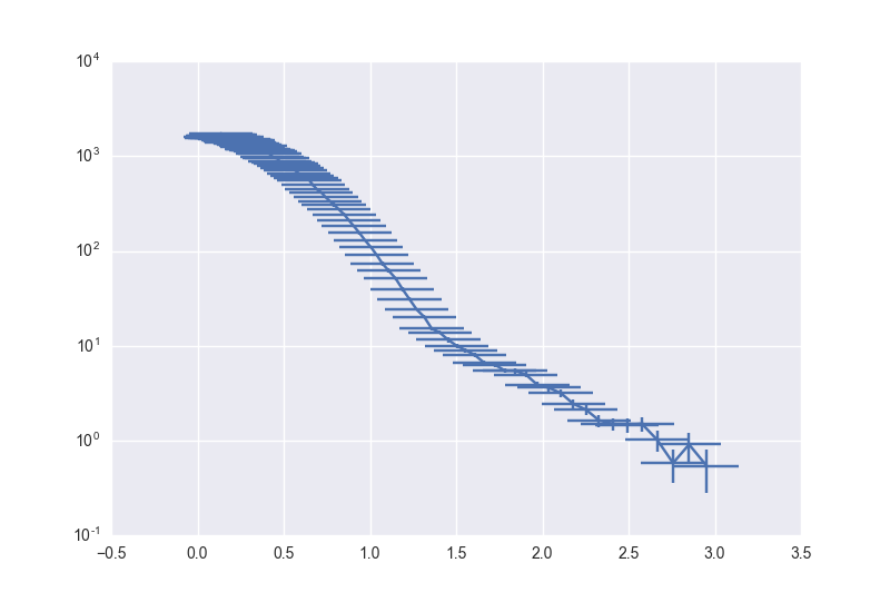
We evaluate the q-uncertainty along the detector of silver behenate by determining the q-position of the datapoint with the largest intensity for each peak. No peak fitting is done (on purpose), as we are trying to simultaneously assess the worst-case practical q-uncertainty between datapoints in this way. Unfortunately, we cannot easily maintain the same binning as for the “standard” dataset (i.e. a goal of 100 datapoints for the range 0.1 – 3 ) as the peaks span a much different range. Instead, we will consider the 3.5% q-uncertainty introduced by the standard binning procedure to be a lower limit of the uncertainty estimate determined herein.

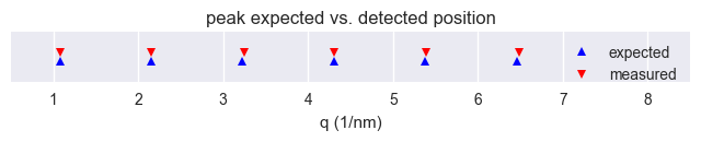
The q-positions of the datapoints with maximum intensity in the silver behenate sample are shown in Figure 4. Figure 5 shows the deviation per reflection.

This result shows that our q calibration is ever so slightly off: the measured peak positions are consistently higher than the expected values. However, this deviation is an order of magnitude less than the position uncertainty introduced by the binning (3.5%), and therefore well within limits.

Apoferritin

Apoferritin is not as popular as silver behenate as a calibrant, but it is more convenient in several ways:
1. Its scattering pattern can be calculated from crystallographic models to good agreement
2. It has a distinct feature (dip) in the scattering pattern at lower q than silver behenate
3. It is very stable, with a well-defined structure in solution
4. Its liquid state means it is easily injected into an existing liquid-sample configured instrument.
5. It scatters quite strongly, requiring little measurement time.
6. It is quite cheap.

To model it, we follow [Zhou-2005, Leiterer-2008] and approximate its structure as a core-shell sphere with an inner radius of 3.75 nm, and an outer radius of 6.2 nm. We then use the pattern-shifting method, explained in the following paragraph, to see how far we are off in our calibration. We apply the same using a CRYSOL-modeled scattering pattern from the published PDB structure.

The pattern-shifting method

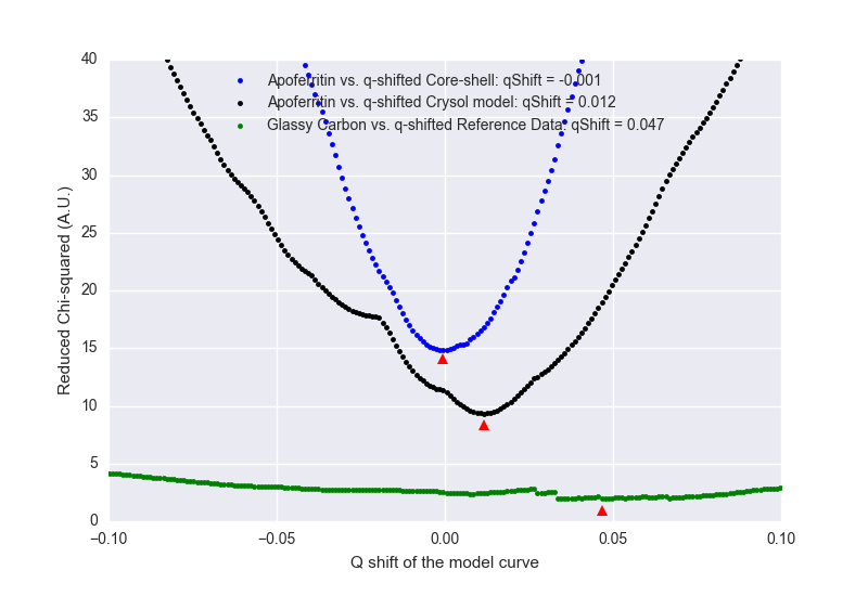
In this method (also introduced here), we take a given measured pattern, complete with uncertainties, and compare it to a calibration dataset. The measured pattern or calibration dataset is shifted by a given amount in q. We then compare the fit of the shifted pattern after scaling the intensity, and calculate the goodness-of-fit parameter . In order to calculate this, we do need to perform a (linear) interpolation on the intensity over q, along with the uncertainties, which can create a bit of numerical “noise” in the result.

For a pattern for which there is no perfectly matching calibration dataset, we can only determine the best-fit q-shift. This can serve as a basic q-calibration method. One remaining way to then estimate the uncertainty on the fitting parameter, is to find the width at . This is a method used in, for example, p.62 of the Ph.D. thesis of Gudrun Gleber.

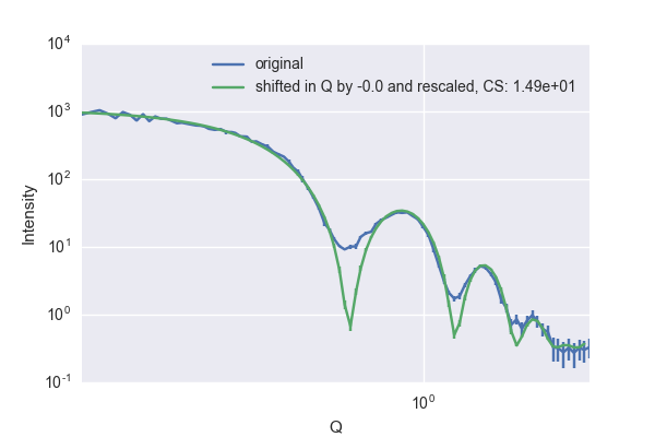
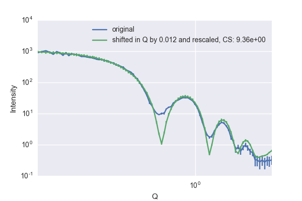
This shift method shows (in Figure 6 and Figure 7) that our data is well aligned to match the core-shell approximation to the Apoferritin model, and confirms that any shift in our q axis is well below the size in q that our datapoints describe, although it is hard to estimate the variance using this simplified model. Similar information is obtained when we apply the same method using a scattering curve calculated from the PDB crystal structure (Figure 8), and although that pattern appears to be shifted by 0.012 , this is more than 50% smaller than the resolution at which the CRYSOL model has been calculated.

Estimating the mean for both Apoferritin fit curves above at the position where , that would be an uncertainty of 0.035 (estimates are 0.03 and 0.04 for the curves).

Glassy Carbon

Of interest is to note that, when we consider all the datapoints as an ensemble, we are very sensitive to shifts of the entire axis. This indicates that we may even be able to use glassy carbon as our calibration sample. Like Apoferritin, we are not using it to determine the sample-to-detector distance, but rather the shift of the entire q axis.

Unfortunately, the results for Glassy Carbon are nowhere near as nice as they could be (Figure 6, Figure 9). The results show that we have a shift of nearly 0.05 , and are still not reaching a . This is far out of line of the results from both the silver behenate as well as the Apoferritin, and therefore we tentatively conclude that Glassy Carbon does not lend itself well to calibration of the q axis. On a positive note, our absolute intensity calibration using water scales the subsequently measured glassy carbon data to within 10% of its reference values.

Evaluation of the worst-case (divergence-limited) scenario

In order to estimate the effect of the divergence-induced shift on the size determination, we shifted the aforementioned silver nanoparticle pattern in q. Two patterns were thus generated, one with a negative shift by half the divergence-induced shift, and one with a positive shift by the same amount.

Note: the fits were performed on a reduced number of datapoints, to ensure the approximate same minimum q is used for the fits (the negatively-shifted data otherwise contains excessively small q values). These results are given graphically in Figure 10.

Evaluation of the calibration-limited scenarios

Another estimate would be using the largest realistic value from the practical q-shift measurements, i.e. the one determined from the shift between the Apoferritin data and the CRYSOL model, which is 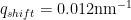. As before, all analyses have their low-q value limited to remove range inconsistencies.

The second calibration-derived estimate used is the shift of , as deduced from the calibration of Apoferritin. These results are given graphically in Figure 10.

Evaluation of the binning-limited scenario

The last estimate uses simply the binning-induced uncertainty in q. As this width is a constant fraction (3.5%) of the scattering pattern rather than a shift, the estimation is done on patterns whose q-vector has been magnified and shrunk by 1.75%.

The effect of this on the results is as follows:

• The mean radius determined from the shrunk, normal and magnified q axes are: 3.267(4), 3.214(3), 3.186(2)
• The width (square root of the variance) of the same, are: 7(1), 6.7(9), 6.5(8)

The binning, therefore, introduces an uncertainty of approximately -1/+2 % in the mean, which is the same magnitude as the round-robin uncertainty. Concerning the distribution widths, the binning appears to introduce an uncertainty of -8/+6 %. This is, however, significantly smaller than the uncertainty in determination of the widths.

Overall uncertainty estimate

The silver behenate measurement shows that we are well within expected values for the peak positions, and so we conclude that the sample-to-detector distance is accurately defined. In other words, we have no uncertainty contributions leading to a shrinking or magnification of the scale outside from the binning-induced effects, and can concern ourselves mainly with the uncertainty in the q-shift of the entire axis.

The binning-induced (smallest possible) uncertainty on the q scaling is on the order of three percent (mostly defined by the datapoint width and the binning). This is superseded by the practically determined possible zero-q shift from the Apoferritin measurement of up to 0.012 . In total, these uncertainty contributions can affect the determined mean radii by about 1%, but the effect on the distribution width is within noise levels (see summarizing figure).

When we consider the zero-position uncertainty as derived from the -behaviour of the Apoferritin models vs. the Apoferritin measurement, we can estimate an uncertainty in the q shift of . This can introduce a maximum uncertainty in the mean radius of up to 2.5%, and in the distribution width of up to 35% in the worst case.

Lastly, the divergence contribution is very large, introducing a potential smearing in the data with a width of almost 0.1 . The effects of such a shift on the radii would be quite dramatic, but we assume that the effects thereof are centrosymmetric, and (largely) compensated by the desmearing procedure in this particular application.

The afmorementioned q-uncertainty contributions can, therefore, realistically affect the determined distribution parameters by up to a few percent for the mean radius, and possibly up to 35% on the distribution width determination (worst case scenario). The latter, however, is hard to distinguish from the numerical noise inherent in its determination.

This uncertainty budget should ideally be recalculated for every measurement. It is expected to be less severe for instruments with a more parallel beam, and a higher data accuracy (allowing for smaller uncertainty estimates on the determined parameter). At the very least, this derivation is a valuable exercise which brings great insight into the instrumental errors which can constrain our technique.