

Just in time for the Copenhagen small-angle scattering summer school of a few weeks ago, we made sure to have a usable user interface for McSAS3 called McSAS3GUI, and I made a video playlist (here) to help the participants (and perhaps you) get started with using it. If you have large quantities of in-situ or operando data, and have trouble getting a model to fit all of it nicely, McSAS3 might be just what you need.
Read on for more details on the MC method, why we made McSAS3, and some tips on using McSAS3GUI…
We talked about it a bit before in this post, but McSAS3GUI is a separate user interface module to help run McSAS3. McSAS3 is the headless, refactored successor to the original Monte Carlo small-angle scattering analysis software McSAS which we published about in 2016 here. The user interface is made to be as friendly as possible, comes with five different usage examples (templates), and can be preconfigured by your friendly instrument scientist to make it as easy as possible for you to use for your large quantities of data.
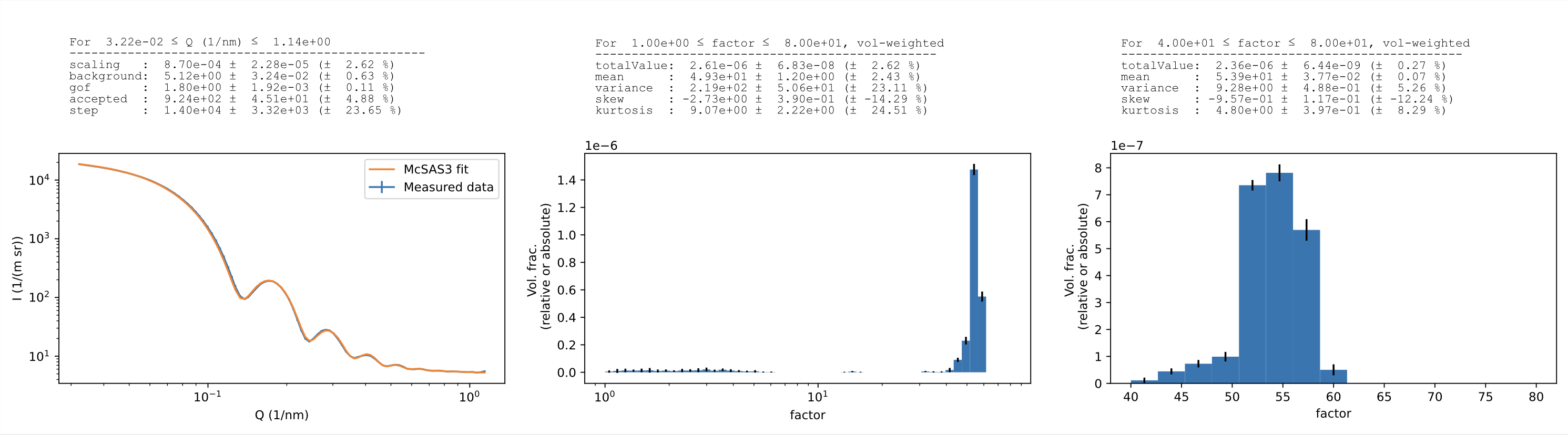
For those who are not familiar with this approach, what the Monte Carlo method does (as explained in this video) is analyse scattering patterns to extract form-free distributions. These can be any parameter distributions in principle, but in practice are usually (volume-weighted) size distributions. It is able to immediately fit a large range of scattering patterns, e.g. from polydisperse particles or pores in a matrix, dense globular particles such as powders, or even more complex systems. It is ideal for following the growth of particle populations in in-situ data, and will quickly give you an indication on the sizes of the population(s) in your sample. Indeed, it has been the workhorse of my analyses…
The trouble with OG McSAS…
While the original McSAS has been used for a large number of papers, it had design issues that were impossible to resolve without a major rewrite. For example, the UI was inseparable from the core, so that headless operation or integration in data processing pipelines was impossible. Secondly, the number of models supported was rather limited, and it did not support multicore processing. Most annoyingly, you could not change the histogram settings without having to redo the complete (and occasionally time-consuming) optimisation.
Enter McSAS3
McSAS3 solved these issues in the following ways:
- McSAS3 was designed to be integrated in workflows, running from the command-line or (with some effort) from inside a Jupyter notebook
- It supports a range of input data formats, either in text format or in HDF5 format. Data read-in options can be specified in detail using a configuration.
- It uses sasmodels under the hood (the models library underpinning SasView), which means that many models are supported as well as some structure factors. Combinations of models can even be constructed using a simple syntax (e.g. “sphere@hardspere+cylinder”).
- Multicore processing was implemented for the independent repetitions, making sure you can now use your computer as a space heater again.
- You can now re-histogram a finished optimisation to your heart’s desire.
- McSAS3 was built in a very modular fashion, making it more maintainable and hopefully a bit more future-proof.
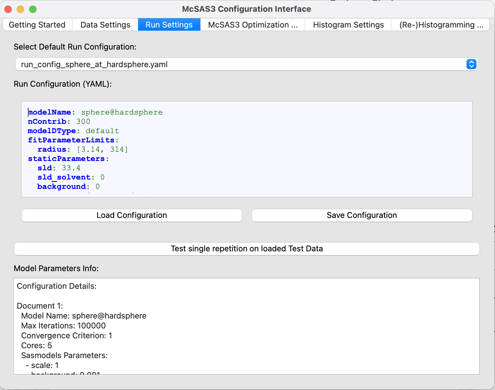
The problem with McSAS3 was that it was not user-friendly enough. Configuration was done using three YAML configuration files, one to specify how the data is supposed to be read in, another to specify how the optimization is to be run (model settings and optimisation settings combined), and the last configuration file specifies how the histogramming should be configured.
We used this for several large datasets but the lack of convenient interface remained a bit of a barrier for the occasional use. Enter McSAS3GUI / M3GUI.
The independent user interface
This user interface does its best to help you configure and run McSAS3. It can be used either as a configuration tool to construct the configuration files, or as a user interface to fit and histogram (batches of) files. M3GUI calls McSAS3 under the hood, and shows you how to call it to help you integrate McSAS3 in your automated data processing pipelines.
To help you get started, there are also prefab templates you can choose from (using a pulldown menu in the “Getting Started” tab), that demonstrate various fits and optimisations by filling in all the required fields in the various tabs. This YouTube video shows the easiest example of this, with more advanced examples available in the playlist.
I made a YAML editor in there that provides some indication when there are errors in the configuration. The information in the editor is also read directly, and a little text box at the bottom provides occasional hints or information on how to proceed. For example, when an HDF5 dataset cannot be found, it shows which datasets are available in the data read-in configuration tab. In the run configuration tab, once a sasmodel is specified, it shows the available parameters that need to be configured.
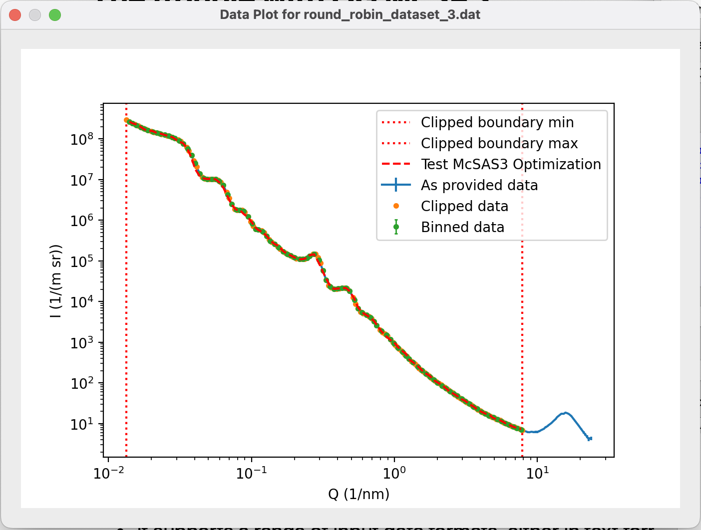
The interface also allows you to test your settings. If a test datafile is specified, and if the data read-in parameters are interpretable, it loads and visualises the data. The run configuration can then be tested on this test data.
For small-ish batches (tested in practice with up to about 5000 files), the UI can be used as well. The “McSAS Optimization…” and “(Re-)Histogramming…” tabs allow for loading a list of files which will be sequentially analysed.
Installation
While we don’t have a precompiled binary yet, the installation of McSAS3GUI (which also installs McSAS3 as a dependency), is not challenging. While there is a video explaining how to install it from source, thanks to my colleague Ingo, it has just become a little easier as it is now a python package that can be pip installed (“pip install mcsas3gui” should install both the engine and the UI).
First steps…
Following the instructions in the “Getting Started…” tab, especially in combination with the videos from the YouTube playlist should make it easy to get some familiarity with it. I do recommend reading the tips and hints below, though:
Some operation notes:
- Due to an issue in the automatic filtering, “background” *must* be set to zero in the staticParameters of the run configuration!
- There is no “stop” button, so it is wise to start with a small maximum number of iterations to avoid waiting too long for it to return.
- If you do not have decent uncertainty estimates on your data, but you want a first look at a fit, it can be helpful to set a maximum amount of accepted moves.
- If you don’t have evidence of your scatterers being any other shape, stick with spheres. This works for most systems (porous systems, elongated scatterers, random structures, fractal structures, etc.), and you will then get an idea on the dimensions of scatterers in your system.
- Stick with one fitParameter to avoid generating non-unique solutions to your scattering pattern.
- Peaks appearing in your scattering pattern that originate from scattering from regular structures cannot be modelled.
- Only sasmodels with a “volume” definition can be used due to the volume weighting of the underlying optimization. the “porod” or “guinier” models, for example, do not have these and will not work. Most shapes do.
- Loaded data is automatically rebinned (default 100 datapoints) to avoid going overboard with the number of datapoints. Uncertainty estimates are obtained from:
- propagated uncertainties, superseded by, if larger:
- standard error on the mean, superseded by, if larger:
- 0.01 (or whatever IEmin is set to, default 0.01) of the intensity in that bin.
Contributing…
Naturally, neither McSAS3 or McSAS3GUI is ever truly finished. If you’re familiar with Python programming, we always welcome contributions, primarily via pull requests. There’s some under-the-hood improvements of McSAS3 that I’d very much like to see done (e.g. shifting to a different data model we’ve started for MoDaCor, to improve data source flexibility, units support and reduction of code duplication), and there are a lot of usability improvements that could be done to McSAS3GUI. Furthermore, we also are trying to get compilation working as part of the GitHub actions. The set-up of the code is made to be as modular as possible to help in maintainability and clarity, and I hope this makes contributions and adaptations easier.
Publication coming soon…
Naturally, everyone will want to use this in their research and cite an appropriate literature reference. The paper for McSAS3+GUI is in advanced stages of preparation and will be submitted before the end of the year.