

A remark in a recent paper by Dr. Yojiro Oba (currently at KURRI) caught my attention. It discusses which shape assumption can be appropriate to fit a scattering pattern of polydisperse systems. In the paper, the shape assumption is spherical (based on TEM evidence), and a further remark goes as follows:
“ Since no q−a (a < 4) behaviour is observed, the possibility of anisotropic shapes such as a rod, disc, and ellipsoid of revolution is denied. ”
That is an elegant way of putting it (note that it is an unidirectional exclusion and does not work the other way), and it sounds about right. So let’s test this with some simulations. These, of course, cannot prove that the statement is true, but can only disprove the statement.
For the simulations, we use the familiar SASfit software (version 0.94.5), whose stability has much improved in recent years. For fitting, we use the McSAS Monte Carlo method. The uncertainty estimates have been calculated using Excel in between the simulation and fitting procedures.
For this test it would be interesting to investigate the three commonly used shapes: spheres, thin rods and flat discs. I want to find out whether any of these shapes can be reasonably described with any of the other models, e.g. if we can fit a scattering pattern from flat discs with a sphere model, and a scattering pattern from spheres with a thin rod model, etc..
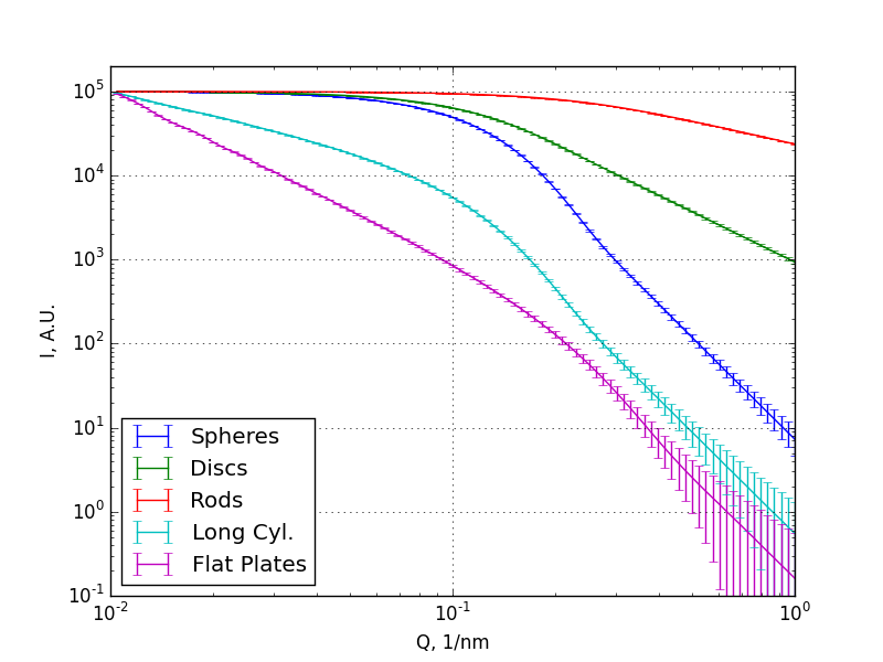
For the sake of clarity, we define a rod here as a long, cylindrical object, with the radius (0.5 nm) well below the size limit imposed by the Q-range (3 nm), and the length distribution within range. We define a disc as a flat cylindrical object, with the radius within range and setting the length (0.5 nm) well below the Q-range imposed size limit (3 nm). The simulation settings are specified for spheres, discs, and rods in the “Simulation settings”-section below ([s1], [s2], and [s3], respectively). The scattering patterns are shown in Figure 0.
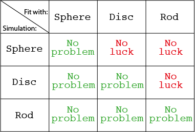
The results (Figure 1) are in agreement with the statement above. We can fit any simulated scattering pattern from rods, spheres or discs using spheres, but not necessarily the other way around. So the statement in the paper appears to hold up for these shapes. This is also evident from the shape of the scattering patterns (Figure 0) where the less sloped curves would be challenging to match to the steeper-sloped curves.
That should have been the end of that story, but I decided to go a little further (a simulation too far, perhaps).
Things might get more complicated with other models (e.g. long cylinders (fitting radius), wide plates (fitting thickness). As a test, I tried simulating long cylindrical objects (see [s4] below), whose length exceeds the Q-range limit, but the radius range falls squarely in it.
From our diagram, we should be able to fit pretty much anything to polydisperse spheres. This model gets there, but only with the addition of a few extra contributions (500 instead of 200).
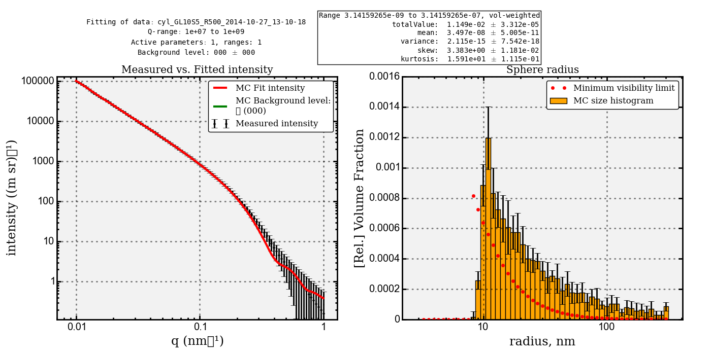
Flat platelike objects ([s5]), on the other hand, can *almost* be fit with spheres, but not quite completely. Whether this is a failure of the simulation, the fitting method or the assumptions, I cannot yet tell. It looks like it should be possible, but the vast span of uncertainty estimates may be reducing the optimization speed of the MC algorithm.
Anyway, I hope this post may encourage some of you to start playing around mixing and matching morphologies of simulation and fit. It is an interesting topic that often comes up when discussing SAXS, and it will be worthwhile to test some more shapes (and it is definitely worthwhile to test your particular sample assumptions!).
A final note of warning: this is simulated data, unaffected by smearing and multiple scattering, and assuming sharp boundaries between the different phases. In real instruments you may actually change the slope of the scattering curve through (a combination of) any of these effects! Always support the shape assumption with data from other techniques, and do not rely on SAXS alone!
–Simulation details–
Q-range: 0.01 – 1 (1/nm), divided over 100 log-spaced points. Intensity normalized to 100000 virtual counts at q = 0.01. The uncertainty is estimated as the square root of the virtual counts or 1% of the number of counts, whichever is largest.
[s1]: FF: Sphere, (number-weighted) R-distribution: Gaussian, sigma = 5 nm, X0 = 10 nm. Remaining parameters = 1.0. Vol-weighted distribution has a mode at ~15 nm, and a FWHM of about 10 nm. 64 datapoints have uncertainties limited to 1% of the intensity.
[s2]: FF: Disc, (number-weighted) R-distribution: Gaussian, sigma = 5 nm, X0 = 10 nm. 75 datapoints have uncertainties limited to 1% of the intensity.
[s3]: FF: Rod, (number-weighted) L-distribution: Gaussian, sigma = 5 nm, X0 = 10 nm. all datapoints have uncertainties limited to 1% of the intensity.
[s4]: FF: Cylinder, (number-weighted) R-distribution: Gaussian, sigma = 5 nm, X0 = 10 nm. L = 500 nm.
[s5]: FF: Cylinder, (number-weighted) L-distribution: Gaussian, sigma = 5 nm, X0 = 10 nm. R = 500 nm.
–Fitting details–
Sphere model R-range 3.14 – 314 nm.
Disc model using “Isotropic Cylinders” with length set to 0.5 nm, and radius range 3.14 – 314 nm. Limited to 31.4 nm for faster convergence where appropriate.
Rod model using “Isotropic Cylinders” with radius set to 0.5 nm, and length range 3.14 – 314 nm. Limited to 31.4 nm for faster convergence where appropriate.
“Asphaltenic aggregates are polydisperse oblate cylinders” (doi:10.1016/j.jcis.2005.03.036) provides an interesting perspective on this subject (not my own work). It would also tend to disagree with the (in my opinion a little too simplistic) statement given in Yorijo Oba’s paper. To summarize, they noted that various different shapes had been used to fit SAS data arising from dispersions of asphaltenes, and analyzed several of their own data-sets using a variety of different models in order to judge the closest match using the goodness-of-fit parameter. In this case information from other techniques was not easily accessible (as is often the case in real systems). I guess the conclusion could therefore be (which I believe still fits with your analysis above) that choosing spheres over short cylinders to fit a single given data-set is potentially equally as misleading as choosing short cylinders over spheres if goodness-of-fit is not accounted for.