Does it matter, part 7: Generator warm-up

Many of my mentors have insisted that the X-ray generator needs some time to stabilize after setting the generator voltage and current. The given waiting times vary from half an hour to about an hour, during which one cannot expect a stable measurement (wasting energy in the process). However, is this really an issue?
To find out, I started a measurement right after setting our old-ish Philips PW1830 to the operating conditions (40 kV, 40 mA). This measurement consisted of 180 repetitions of 10 seconds. The final Anton Paar .pdh file is pretty useless, as it has averaged the data over the 180 repetitions, but fortunately they supply a .tif image file.

Upon closer inspection, the Anton Paar Tif file contains the raw data from the measurement (in counts). The image is a multi-frame .tif image, with one frame per repetition. Fortunately, reading this image appears to be problem-free, although since the image contains only 16-bit values, and the Mythen detector can store up to 24 bits in its registers, I wonder what will be stored in the .tif file if the amount of detected counts in one pixel exceeds 65k…

Anyway, back to the problem at hand: do we see any evidence in the patterns that would support the practice of “warming up” the generator? Let’s start up Python and see what we get…

Data Read-in

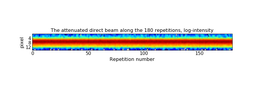
We can read in the .tif image that is produced when we ask our Anton Paar SAXSess to measure 180 repetitions of 10s frames. For this, we use the “Pillow” library, which is an image library that can read a variety of images. We extract the individual 1-by-1280 pixel frames and put them alongside (figure 1).

This looks fairly uniform over time, with no obvious time-dependent beam shifts or drastic intensity variations. Let’s take a closer look at the intensity.

The beam intensity

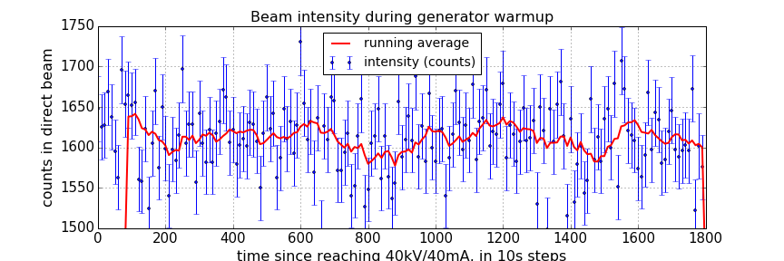
We now look at the summed counts in a given image over these 15 pixels. At the same time, we plot a ten-sample running average to get a better idea of possible trends (Figure 2).

From the looks of it, there appears to be little to no trends in the beam intensity over time. The running average does show some fluctuation, but whether it is significant or not is hard to tell.
One way of determining whether the deviations are significant is to use our good friend: the Poisson distribution. If the fluctuations we are seeing are just due to the counting uncertainty of random events, all the counts should fall within a Poisson distribution. If, however, there is an additional contribution to the fluctuation, for example an effect from warm-up or other generator-instabilities, then the distribution of counts should exceed that of a Poisson distribution.

The Poisson distribution:

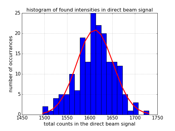
Histogramming how many cumulative counts we have in the fifteen pixels of each of the direct beam images gives us the data shown in Figure 3. On average, we find 1612 cumulative counts in the fifteen pixels. We can use this value to plot the Poisson probability mass function for a this mean value. This probability mass function gives us the likelihood of finding a particular number of counts in a single sample for that mean.

As we see, the Poisson probability mass function very nicely describes our data, and there is no indication that any of our findings are due to any other effect. That means that with these experiments, we have not been able to demonstrate the existence of a warm-up effect.

So for now, until we have evidence to the contrary, we may as well save ourselves some Joules and time, and start measuring right after getting our generator up to power. The same may not hold for other generators, but this is an easy method for checking it for yourselves.

Here is a handy PDF document of the above, but with extra comments and the exact python commands to replicate.