A database! Helping you make sense of the soup in five years.

Two weeks ago, @tostri asked:

tostri @drheaddamage I wonder have you gotten any further with your analysis of JuilaBase? 18/01/16 17:35

which is a valid question. A while ago, I was trying to find out how to keep track of measurements and samples, with a simple goal: a few years from now I want to be able to retrieve the measurements I do today. This requires a database to keep track of measurements (such a LIMS, incidentally, will also enable other advanced analysis, troubleshooting and tracking tasks).

Some options for such databases include JuliaBase, ISPYB (to which Nick Terrill alerted me recently), or we can “roll our own”. Here is what we did…
Firstly JuliaBase. This appears to be a valid option, with a seemingly well thought out user interface, and fine-grained access control for the users. When I looked at that a while ago, however, I could not make sense of the structure of the program at a glance, and therefore could not figure out how to adapt it from its primary purpose (keeping track of surface-deposited samples) to our purpose (keeping track of our sample and measurement information, and mining it for data corrections).
It is probably possible to do so, given sufficient time and investigations, but I could not figure it out fast enough.

ISPYB is a database system in use at some European synchrotrons to keep track of biological samples. It seems to be well integrated in these places, with options to find out what the measurement status of samples is and what the data looks like. Unfortunately, the code is difficult to access with the website stating:

The ISPyB project itself containing trackers, issues, bugs, wiki, and sub-projects as Dewar tracking and BioSaxs, can be found on http://forge.epn-campus.eu/projects/ispyb, but it is a private project, only shared with current developers.

Such messages are not particularly inviting. I did manage to take a peek at the internal structure in the documentation here, which convinced me that this is a set-up which is particularly geared to its biological purpose, and would be a terrible pain to adapt to our much more simplistic needs.

So I needed something flexible that would suit our laboratory, and which, if needed, could be easily converted into various other database forms if we decided to change to something else later on. Most of all, I decided to embrace my inherent laziness and to use as many readily available packages and methods as I could.

And so laziness dictates:

• Information storage / data safety: one file per information item (entry). The database must be able to be reconstructed from these base files.
• Information input: Well, we already have perfectly suitable text editors (and each has his or her preferred one), and the YAML format, while not the most widespread, is easily understood.
• Information management: Users can easily copy entries, delete entries and move them about as each entry is a file…
• Information read-in: Python has a YAML reader, which can pipe its data into a Pandas DataFrame. The benefit is automatic sensing of data types, and on-the-fly definition of column names based on what is stored in the YAML file.
• Information display: for now, read-only HTML tables, and a nice utility called “pivottablejs” which turns the pandas tables into a javascript table, with bar graphs, selectable fields, etc. (this turns out to be a Really Useful Thing, allowing us to do 90% of the searches we need to do).
• Flexibility: Since various measurement methods will each have their own set of data, adding optional fields of information must be easy. This flexibility is inherent in the Pandas set-up.
• Flexibility II: As mentioned before, if the database system needs to be merged into something else at some point, I want that to be possible (i.e. not tied to a single system). This means that the information must be present in an easily translated format, from which the database can be re-built in any alternative database flavour.

So what remained was to make a smart separation. Our data is separated in the following directories (c.f. Figure 1):

1. organizations: Each file / item contains information (addresses, etc) of an organization
2. persons: the same for people, with links to the organizations they work at.
3. photos: a directory for photos of samples, instrument components, people, etc.
4. instruments: one item per instrument, where it is, who is responsible, etc.
5. instrumentOptions: Things like optional sample stages go here, as do all other items that may be combined into  an…
6. instrumentConfigurations: An instrument configuration combines the instrument options (through a relational table) into a single set-up. In the instrument configuration we also find the alignment information for slits, beam positions, etc.
7. sampleContainers: Here, items such as borosilicate capillaries, flow-through cells, etc are listed.
8. samples: one item per sample, describing where it is, who is responsible for it, who owns the sample and how the sample should be disposed of.
9. measurement: This is the big one. Here, the following is combined: an instrument configuration, a sample, a sample container, and a (group of) operators. In the measurement information we also find, for SAXS at least, things like transmission factors and links to background measurements. We also store the measurement files together with the database, linked from here.
10. analyses: Eventually, we would like to associate a particular analysis with a measurement or group of measurements. This information goes here.
11. reports: A (group of) analyses can be used to make a measurement report. The details can be traced back from this point all the way to the organization to whom the sample(s) belonged to.

What do these files look like? Well, let’s look at a (made up) sample description file:

 

---
sampleID: s20160122011 
owner: janpieteman 
ownerSampleRef: BP186
sampleNotes: oil in water with surfactant, 
receivedDate: 2016-01-21 09:00:00
projectName: Structure in liquid 
plannedMeasurements: SAXS, UV-VIS, DLS
localResponsible: brian
receivedImageFile: photos/p20160122001.png 
treatment: return 
chemicalInfo: C20H42 in H2O 
shelfLife: 2016-06-01 09:00:00 
disposalDate: .inf 
disposalInfo: normal waste 
condition: liquid 
storageCondition: ambient 
storageLocation: H20 R112 Brian's sample cupboard 
storageOrganization: bam

This datafile can be directly read by both humans as well as python, and the data types (date, string, etc.) are automatically determined. This then specifies a sample quite completely, and has links to the people (linked to the people table) responsible for aspects of the sample. It also has a link to a photo so you know what the sample looks like visually if you have to search for it.

We have similar information files for all the other aspects (measurements, instruments, instrument components, etc.). Let me show you one more of interest, the measurement file:

---
measID: m20160122016
instrCfgID: ic20160113001
opGroupID: op20160105011 # This is brian by himself!
sampleID: s20160122011 
sampleReusedFrom:
logbookID: S1234
rawDataFileLocal: 'C:\Data\brian\S1234.tif'
rawDataFile: 'measurements\saxs01bam\S1234.tif'
processedDataFile: 'measurements\saxs01bam\S1234.pdh'
smearedDataFile: 'measurements\saxs01bam\S1234.pdh'
background: m20160122006
sampleContainerID: sc20160121001
measQuality: 2 # 0: not determined, -1: Rubbish, 1: usable, 2: Super
measNote:

# following this is a list of data reduction parameters: the 
# schema of the imp2 data reduction methods. Items already
# defined in instrument configurations do not need to be redefined
sac: capillary
tfact: 0.35 
time: 10 # measurement time for a single measurement
repetitions: 120 # Number of repetitions
tstamp: 2016-01-22 14:01:00
flux: 1.0
temperature: 294.15 # Degrees K, 294.15 is 21 degrees C

 

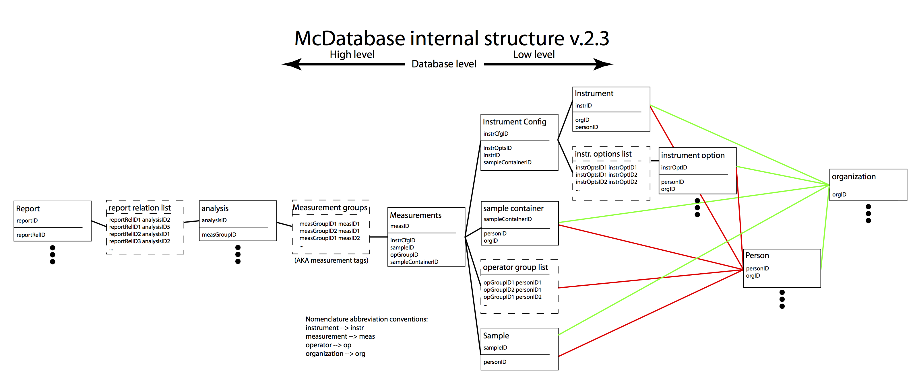
These entry files in the aforementioned directories then form separate tables of information, which are linked in the way shown in Figure 1. Using pandasql, we can perform searches in the linked tables using the SQL syntax. Many database people will be familiar with this language, and happy to have its power at their disposal.

Right now, we are putting the system through its paces, filling in the data as we do practical measurements, make changes to the instruments and so on. Gradually, we are discovering that some information is best left in other files (sample containers, for example, should be part of samples, and not instrument configurations), and other information is missing (what if we measure the same sample-in-capillary a month later? Can we distinguish between those and freshly loaded samples? Would it be possible to write immediate quick evaluations in the measurement data?).

So far, the team is quite enthusiastic about filling in the database. This was helped by access to the database tables a few days after we started filling in all the data, so everyone could see the fruits of their efforts (these tables are generated a few times a day using a simple python script on the raw files). Additionally, putting the database on a networked drive allowing people to easily access and edit the most recent set of files also helped. Right now, filling in the data is still raises surprising issues, but we are quickly finding our groove.

The next step is to include more instruments in the database, such as a UV spectrometer and a DLS instrument, so that we can trace what measurements have been done on particular samples that have passed through our lab. Additionally, this database may tie in with the data correction methods, providing the parameters for the data correction. Once this automated data correction method is in place, maintaining the database will be easier as well. In that case, much of the file information (where is the smeared data, where is the desmeared data, etc.) will be automated.

I’m curious to see how far we can take this concept. Given enough time and effort by all involved, the results should prove very useful a few months down the road!