

[this is an excerpt from the talk I gave at TechConnect]
Recently, the European Union has defined what they consider to be a nanomaterial:
“A natural, incidental or manufactured material containing particles, in an unbound state or as an aggregate or as an agglomerate and where, for 50 % or more of the particles in the number size distribution, one or more external dimensions is in the size range 1 nm – 100 nm.”
Based on this definition, they want industry to at least label their products as nano or not, and, based on SAXS measurements in our lab, more products are nano than not (graphene, interestingly enough, would not be nano, as the smallest size is below 1 nm, and the largest sides of the flakes would be above 100 nm). There are some practical issues with the EU definition, but I asked, and it is unlikely to be modified. Therefore, it is up to us to live with it for now, and try to measure what they defined. Let’s take a close look:
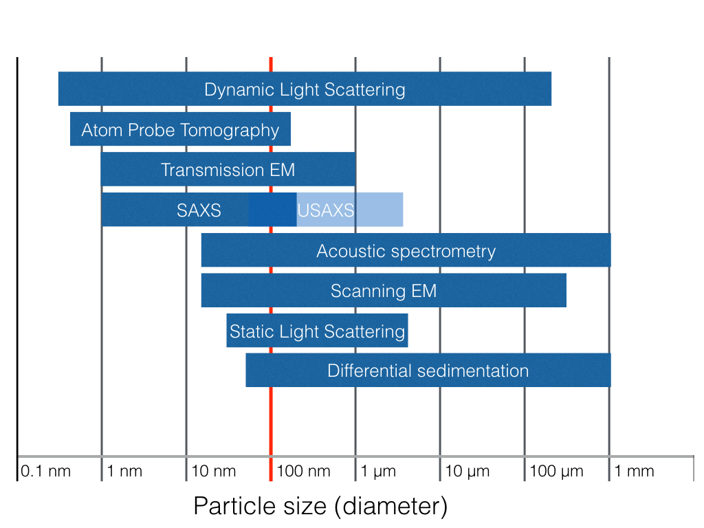
Looking at the available characterization techniques I could find, (Figure 1), we see only a few candidates capable of spanning the range from 1-100 nm. These candidates are quite different in terms of what and how they measure, and so some differentiation might be appreciated.
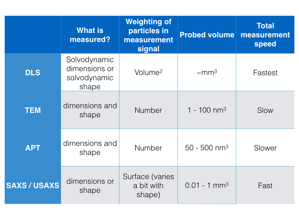
Figure 2 summarizes some of the aspects of the measurement techniques. As is obvious, each technique has its own benefits and drawbacks, and there is no one single omnipotent technique. Note, apropos, that none of the techniques are suited for measuring aggregates or agglomerates. In reality, you need to apply (almost) all of these techniques applied before you can do proper particle sizing. That is a very expensive proposition, so many labs focus on a subset only. We focus on SAXS and DLS in ours.
SAXS is a straightforward technique in theory. In a handful of cases, it’s as easy as it sounds: you insert your sample, collect your scattering pattern at the other end of the instrument, fit the scattering pattern to a model function and out pops your size distribution. Any kid can do it. But nano-metrology is hard. With every technique, in 90%* of real world cases, you run into metrological issues.
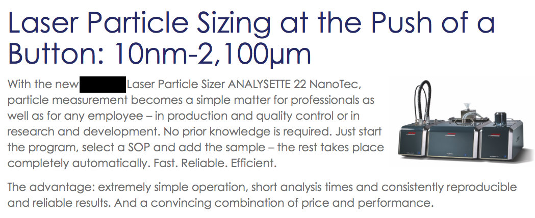
Recognizing when you have issues is essential. Therefore, I am greatly concerned about the recent** emergence of black-box instruments that hide such issues behind a slick front. See, for example, the ad in Figure 3, and feel free to be slightly offended at the linguistic foible separating employees and professionals. The key sentence is “No prior knowledge is required”.
The problem with this approach is elegantly summarized by Feynman in his 1981 Horizon interview:
… now, I might be quite wrong, maybe they do know all these things. But I don’t think I’m wrong. You see, I have the advantage of having found out how hard it is to really know something. How careful you have to be about checking your experiments. How easy it is to make mistakes and fool yourself. I know what it means to know something, and therefore, I can’t… I see how they get their information, and I can’t believe they know it! They haven’t done the work necessary, they haven’t done the checks necessary, haven’t done the care necessary! I have a great suspicion that they don’t know that this stuff is… , and they’re intimidating people by it. I think so. I… I don’t know the world very well, but that’s what I think.
That quote was about nutritionists, not black box instruments, but the point stands: it is hard to ensure you’re not measuring artifacts, and even if you don’t, that you are getting the complete picture. In particular relying on one technique is a recipe for misinterpretation, but so is applying multiple techniques with prejudice. It is so very hard to avoid bias, but that is the essence of science: to measure and detect with a minimum of assumptions, and to approach all measured data critically.
In order to be critical, we need the tools that allow us to be critical. For this purpose, we developed the McSAS software: software that allows you to assess morphological dispersity from your SAXS patterns with a minimum of assumptions. It may not be the approach you want to apply to give you your final numbers, but it gives you a good start at interpreting your data. […] What we found out, however, is that it will fit good data, giving you good results, but it will also fit bad data, giving you shit results. Garbage in, garbage out.
So we worked on getting your input data as good as possible, which meant data corrections. I summarized the lot in the “Everything SAXS“-review paper, and by now it has accrued over 60000 downloads. And this gives me hope, it means that others are also interested in getting their data correct! We will see, however, how far we still have to go when the Round Robin data is evaluated.
*) statistics carelessly extracted from thin air.
**) I’m old.
Leave a Reply