Scattering from arbitrary objects, part 2: fine-tuning the method

It’s been a while since part 1 of this story, but that doesn’t mean development has stood still since then. Here’s what we’ve done…

Introduction

This piece of code will calculate the scattering pattern for any structure, defined in the common STereo Lithography (STL) format. STL is a format that describes the surface of an object, and is commonly used for 3D FDM printers. Its common nature means that structures can be easily drawn by the researcher using their favourite 3D drawing tool, after which this code can do its job.

The underlying code uses the Debye equation, as defined in 1915 by P. Debye (doi: 10.1002/andp.19153510606). This is one of the most fundamental scattering equations, requiring only a number of points to be found within the object.

The next version of this program will scale the intensity in accordance with the volume of the object. As it is now, the intensity is scaled to 1 at q=0.

Details

This code calculates the scattering pattern for a given struture using VTK. The structure is defined by an STL file, which is a standard output format for many 3D drawing programs. The STL file contains no units, so we define 1 STL unit to be 1 nm. This needs to be taken into account during the 3D drawing stage.

Due to the VTK python bindings only being properly and/or easily installed in Anaconda, we are limited to that.
We are following some of the instructions on https://pyscience.wordpress.com/2014/09/03/ipython-notebook-vtk/ with regards to importing objects in STL format, and finding out whether points are inside or outside a closed hull. We then use the Debye equation for points to calculate the scattering function. Initially, a second intensity calculation was performed using the p(r) function, but this was found to give less representative results in a less efficient way.

The Debye equation for single point-pair-distances d: 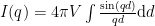$I(q) = 4 \pi V \int \frac{\sin(qd)}{qd} \mathrm{d}d$ .

Improvements since last time

In the previous versions, the q-scale needed to be multiplied with a factor $2 \pi$ , and I didn’t understand why at the time. I since found out that the sinc function I used in the code uses that factor internally, and so it needed to be corrected for. Problem solved.

I also sped up the code through some optimisations here and there, although it still takes several minutes to calculate something decent. Apart from that, I’ve cleaned up all the other attempts and code variants, decluttering the code.

Step 1: Checking the code

Figure 1: Sphere simulation vs. Rayleigh function

Our first step is to verify that the code calculates as expected. This is done using our beloved friend: the sphere. This sphere is defined with a radius of 1 nm (a diameter of 2 nm). We compare this with the Rayleigh function for a sphere of the same radius.

No problems there, only a bit of noise towards high q. This is to be expected as the high-q region relies on points being close together, of which we have only a precious few in a randomly picked case.

Step 2: anisotropic shapes.

I checked the output for other shapes as well, including cylinders and ellipsoids. I highly recommend doing these checks for any simulation, to ensure that this works for anisotropic objects as well (when I used a calculation based on the chord distribution function, this is where that one went wrong). In that case, you would compare the simulated data, stored in the output (csv) file, with the corresponding model in (for example) SASfit.

Step 3: interesting shapes.

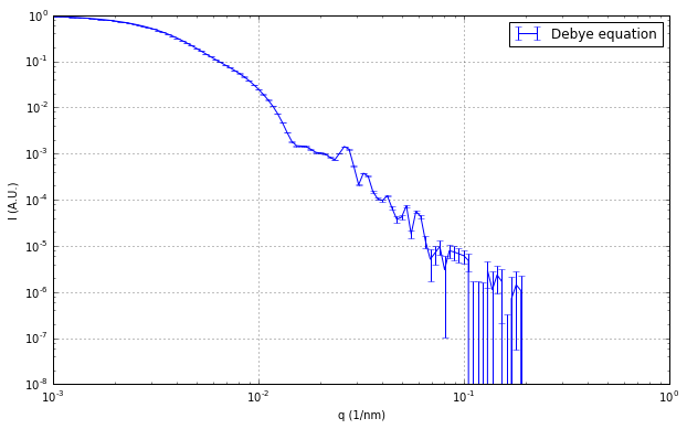
If we'd build an ultra-USAXS around the Brandenburger Tor, this is what we'd see. — Figure 3: If we’d build an ultra-USAXS around the Brandenburger Tor, this is what we’d see.

For now, we’ll switch to an interesting object: the Brandenburger Tor (source: http://www.thingiverse.com/thing:500506). This object is a bit bigger than a 1 nm sphere, so we need to shift q a bit. The limits show that the object spans about 1400 STL units, so in our simulation, that would be 1400 nm. 2π/1400 would give us a lower q limit of 0.0045, which we can reduce a bit to get a well-defined Guinier region. The max. q is a bit limited due to our typical sampling distance (2000 points spread out through that space tend to be quite far apart), so we should probably stay within 2 decades: 0.45.

Given the intended reduction, we’ll do 0.001 – 0.2. See Figure 2. In reality, the BB tor is a bit bigger than 1400 nm, and so we’d expect the q-range to shift by another 7 decades or so for the real object. I also suspect there will be minor complaints, when I irradiate the Tor with a 50m diameter coherent X-ray beam, using a satellite or two as detectors.. Those Berliners do tend to complain at every opportunity, though, they’re almost like the Dutch!

Next steps

This will need just a bit more fine-tuning, and moving from a jupyter notebook to a small Python program. I’m also trying to get this to run under Python3, but VTK isn’t available for the 3.6 version I have yet.. VTK’s a bit of a problem, and one I’d prefer avoiding, but at the moment it appears to be a necessary evil. There are some other improvements to do, and then it’ll hopefully be ready for use in a real project. If you have a shape you need to have calculated, do let me know. Also, if anyone has a suggestion about how to improve the high-q behaviour, I’m also very keen on hearing about that…

Looking At Nothing

A SA(X)S Weblog