SAXS and USAXS, and smearing in McSAS

We got some initial results of the sequential SAXS/USAXS experiments we did at Diamond*I22 earlier this year, measuring one of Zoë Schnepp‘s carbon catalysts. Unique about these measurements is that there is a particulate feature in the sample, with dimensions in the overlapping region between the SAXS and USAXS ranges, so we can compare!

If you forgot what the USAXS test experiments were about, here’s the post that discussed those. During the USAXS tests, we also tried to measure the same sample sequentially using USAXS and SAXS, so that a wider Q-range — and therefore a correspondingly wide size-range — could be probed.

We measured a few samples this way, and we had at least one sample with structural dimensions that could be measured both with the SAXS as well as the USAXS instrument. This allows us to compare the results from both instruments, and see how well they compare. This comparison helps us to validate the correct functioning of the USAXS instrument. There is, however, one tiny snag: smearing.

The Bonse-Hart principle behind the USAXS design implies that we are getting so-called slit-smeared data, fundamentally different than the nearly-unsmeared pinhole SAXS data. Traditional methods of dealing with slit-smeared data include desmearing; a mathematically ill-posed procedure that results in increased noise and potential artifacts, but does allow merging of the USAXS data with the SAXS data. We follow the neutron scattering community in analyzing the smeared data by smearing the fitting model instead. Smearing the fitting model is mathematically robust, and does not increase the noise in the measured signal. The downsides to this are that it does not allow a pretty merging of the SAXS and USAXS data, and that the fitting software must have the capability to smear results.

A while ago, Ingo Breßler and I implemented a smearing method in McSAS. It has not been thoroughly tested yet, and so I have been hesitant to use or promote it. SasView, however, can now export a model scattering pattern in smeared and unsmeared forms, and this allows me to test the smearing implementation in McSAS. Thus said and done, initial tests failed to prove the smearing implementation wrong. That means we can continue using it for the real data!

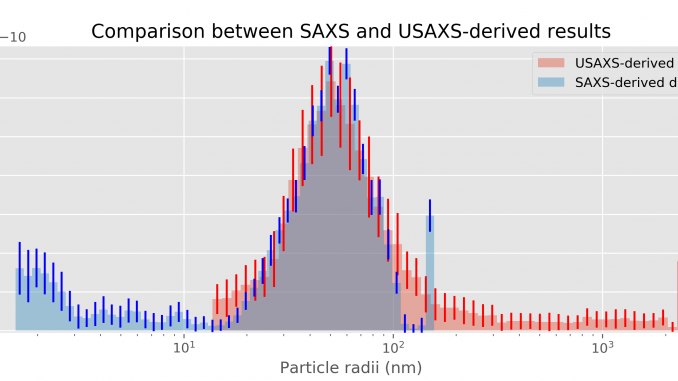
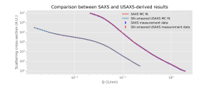
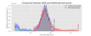
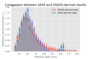
The MC fits to both SAXS and (slit-smeared) USAXS datasets are shown in Figure 1. As usual with the MC approach, the fits are perfect. The resulting size distributions for both instruments are shown in a single graph in Figure 2. As we did not measure in absolute units for these datasets, a scaling factor was estimated between the two, and the volume fractions are given in relative units only. The feature around 100 nm does show up nicely in both datasets. A close-up comparison between the two (Figure 3) also shows a nice agreement. The last bin in both datasets is an artifact arising from the MC method trying to describe a “large scatterer”-background. The sample in this case was a powder, and so the surface scattering from the particles induces an background in the SAXS data, and an  background in the USAXS data, described by this large scatterer contribution.

So, the SAXS data shows us that there is a population of 100-200 nm particles in the sample. The USAXS data not only confirms this, but also informs us that there is no further contrasting structure between 200 – 2000 nm. Together, the two methods provide information on the structure in the sample from 1.5 – 2000 nm. If we can get some decent signal from the WAXS detector too, this would extend the lower end to several Ångström too, but the geometry didn’t allow that in this case. Next time, perhaps.