

Besides the ongoing instrument migration efforts, we are also continuing work on “real” science. One of these involves the backbone of squid (called a squid pen or gladius). These backbones consist of an intricate hierarchical structure which is interesting to investigate. So Melika Moradi, a master’s student, has been put on the task of finding out more…
What to do?
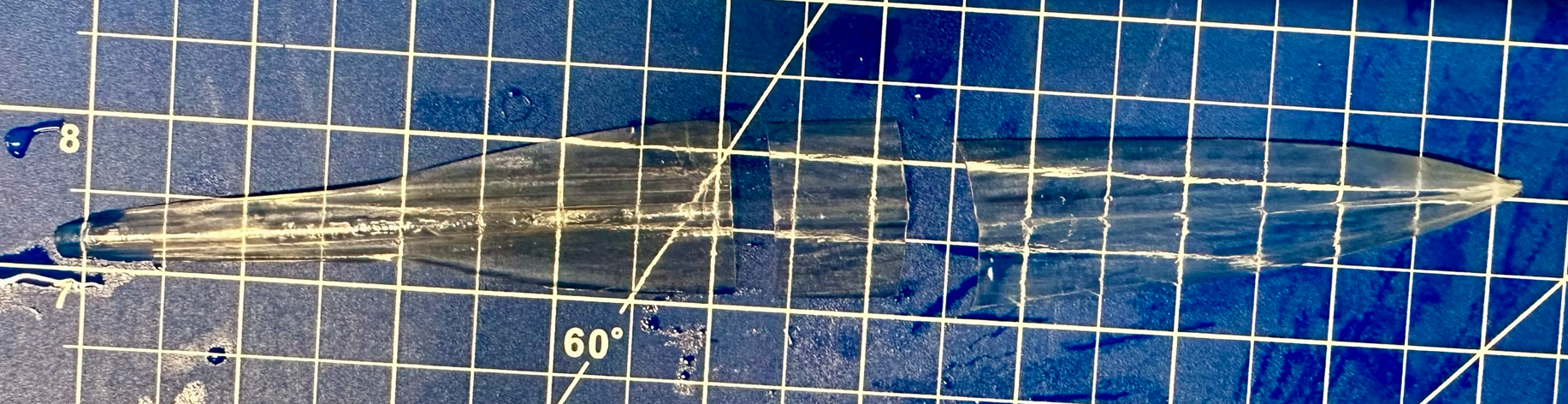
Squid pen get their name from their look: they resemble those old-style feather-based ink pens (Figure 1). They are flexible, clear elements that help support the body of the squid, and are built up from a layered structure of biopolymer (chitin and protein). While some research has been done on this structure, some of the finer details remain unknown. For example: can we locate the protein in the structue, and are there local differences in the structure?
These questions were posed to us by a researcher at the University of Bologna (who also supply the squid pen), so to investigate this, we use our favourite tool: X-ray scattering 🎉! This should be able to give us information on the fibrillar structure in the wide-angle range, and information on the protein structure from the small-angle range. There are several practical challenges to overcome, however.
Drying
One of the biggest challenge is that the squid pen is wet, but we measure in vacuum. Therefore, we need a good way of drying the squid pen without destroying its fine structure. In our labs, we have a few options for this: air drying (optionally in a dessicator), freeze drying (lyophilization), and supercritical CO2 drying preceded by a solvent excange with ethanol. The first step was to compare the effect of these three on the scattering pattern, and also to find a drying method that least affects the shape of the sample as some methods tend to cause shriveling up of the material.
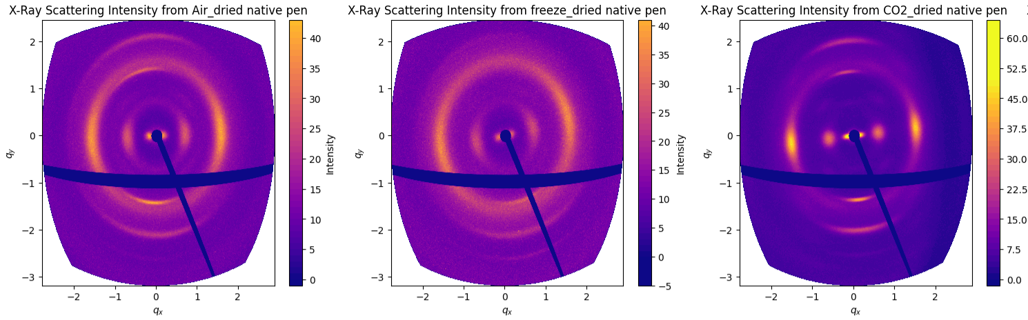
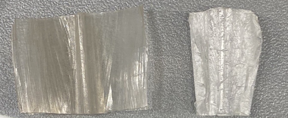
When we compare the wide-angle scattering of these three options (Figure 2), there are indications that air drying and freeze-drying both destroy some of the orientation in the structure (by the broadening of the arcs in the azimuthal direction). Supercritical drying is generally considered to be the best way of drying sensitive structures such as butterfly wings and micromechanical devices. Without more in-depth comparisons, we cannot be fully certain, but it would probably be safest to use supercritical drying for this project given the differences we see. The only downside is that we cannot fit an entire squid pen in the drying machine, meaning we have to cut it up into strips as shown in Figure 1.
Note, by the way, that the display method of the data in Figure 2 is the right way of showing 2D wide-angle scattering data on a Q axis. As the corners of the detector are much further away from the sample than the center, their q value isn’t nearly as far out as a normal 2D plot would show. This distortion would reduce as the detector is moved further aft, but I still think it is cool to see.
Funny shape
The second challenge is that the squid pen has a funny shape. its cross-section looks like a squashed letter W (Figure 3). Ideally, we would be measuring this sample with the material perfectly perpendicular to the X-ray beam, and always at the same distance to the detector. Flattening it between two holed sheets would not be an option as it would impose strain on the structure and therefore would change the very thing we want to investigate. Keeping its shape, however, would mean that we would need to position and rotate the sample around at least four axes. Currently, we do neither, we just scan through the sample and take the non-perpendicularity as given, but if we were to address this, the solution might involve a robot arm!
We have a tiny Mecademic MECA500 robot arm that is small enough, and could hold the sample in the vacuum chamber and position it just right. This would solve our problem, but create a few more. Firstly, the arm is not rated for vacuum, although the company reported that someone successfully applied one in there. If we keep an eye on the temperature, and depower it when needed, we might just be fine.
The second issue to resolve is that of detector safety. Smacking a robot arm through the 100kEuro detector would not be a good idea, and robot arm motions aren’t guaranteed to be logical. So we bought an Omron light curtain normally used to protect digits and limbs from entering moving parts. This, too, is not officially vacuum-rated, and they were not cheap, so I will have to be clever when connecting them. Mounting and connecting these, however, has unfortunately fallen a bit by the wayside due to the hardware issues and migration, but we hope to resume this attempt soon.
A third issue is that the movement of the robot would ideally be informed through a 3D scan of the sample. That part we have not gotten working yet at all. Without that, programming will be tedious.
Once the robot arm and the light curtain are installed, testing can begin. We will let you know, because it may look absolutely stunning!
Analyzing the scattering pt. 1; making the model.
Melika’s project still has a few months to go, but there has already been some success in making sense of the scattering at wide angles. This scattering is full of peaks or arcs. The normal way of analyzing anisotropic 2D scattering patterns is to slice and dice: performing integrations over pie sections or arcs to extract 1D information to analyze. But you are throwing away a wealth of information if you do, indeed a whole dimension! So we set out to do the analysis in 2D.
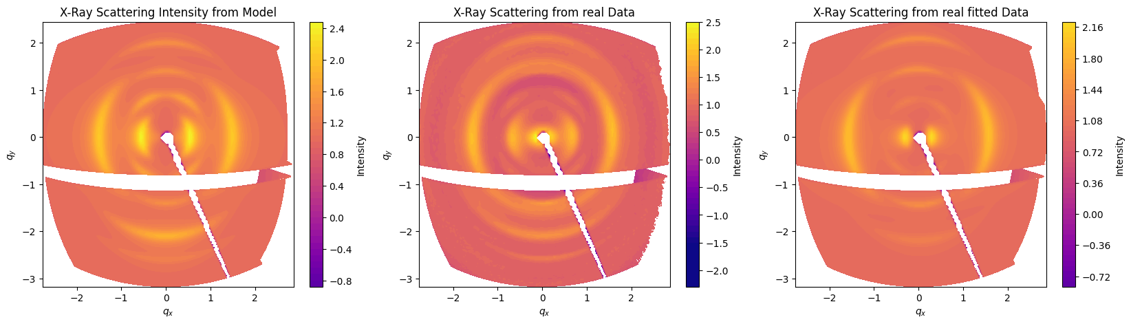
2D scattering pattern analysis can be a challenge: the data can contain 1 million datapoints, and models don’t exist out of the box. The wide-angle scattering contains at least 13 arcs, each with at least six parameters (amplitude, azimuthal position, radial position, azimuthal width, radial width and peak shape), to which an overall flat background was also added. After some time, Melika constructed a 2D model that contained all the peaks in approximately the right position, thus creating a starting point for optimization. Calculation time was fortunately acceptable at a few seconds for each iteration of the ~1M datapoints.
Analyzing the scattering pt. 2: optimization strategies.
least-squares fitting
The most common approach for parameter optimization is using a least-squares optimization algorithm like Levenberg-Marquadt. This resulted in the reasonable fit shown in Figure 4. The only downside is that optimizing 66 parameters in this way (5×13 + background) is not efficient at all, and might not even work well. Secondly, the two equatorial arcs that were in the initial guess have shifted inwards in the optimization to describe the small-angle scattering intensity instead. So this may need some adjustment. I am surprised that it is still working despite the number of parameters, and this approach might warrant a second look
Bayesian optimization
Theoretically, a well-configured bayesian optimization might be more suited to optimization problems with oodles of datapoints. Using PyMC, Melika was able to get a few peaks to optimize, so there is a start. The PyMC approach, however, is resource intensive, and therefore is even less efficient so far than the lmfit approach, especailly when the initial guess is not so good. We have only just gotten started on this problem, however, so we will keep plugging away at this approach. There might be other approaches to fitting such data with many parameters (without azimuthal or radial averaging), so if you know of one, please let us know!
Future plans.
While good progress has been made so far, the project is far from done. Some of the remaining steps include:
- Analysis of the small-angle scattering pattern. The small-angle scattering signal really only appears in the deproteinated samples, indicating that the proteins may occupy oriented void spaces between the chitinous skeleton. This should be modeled, however, and perhaps we can get some correlation between the wide-angle orientation and the small-angle orientation parameters.
- Simultaneous fitting of the wide- and small-angle data, perhaps exploiting links between orientation parameters might be both cool, as well as useful. We will let you know if we can get this working.
- Robots.. yay or nay? Integating the robot in the sample chamber to hold the sample is one thing, getting it to work over days or weeks moving a non-uniform sample around is another challenge altogether. Perhaps one better suited to a Ph.D. project..
- Mapping the squid pen, both the original one and the deproteinated one is essential to answering the question from our collaborator in Bologna. This is high on the priority list, and through analysis of the data we hope to be able to answer this before the end of the project.
In conclusion, this is a large challenge, but it has all the cool bits inside: practical and computational challenges, a cool organism, interesting scattering and some relevant questions. Please wish Melika the best of luck trying to solve this!