

Now that we’ve squashed most gremlins from the new EPICS-ified set-up, we are starting to obtain our datafiles again in the thousands. So far so good, except that nobody in their right mind will want to process these raw pieces by hand.
So it’s high time to get the automated data processing pipeline to work with the new data, and perhaps implement a few quality improvements along the way. Read on for the details on what we do with our raw data and which issues we are trying to resolve.
Why?

In our MOUSE lab at BAM, our primary selling point is the quality of data. Our users come looking for trustworthy answers, and so we obtain these for them (and sometimes with them for in-situ experiments). That means we must concern ourselves with all aspects, from sample planning and preparation all the way to data analysis and interpretation. This “holistic scattering” is a lot of work, but it is a reliable way to make good science available to the material scientists that need it (compared to those who don’t need it…).
As such user support falls squarely on my shoulders (with the occasional help from my friends), exploitation of as much automation as possible is absolutely essential in this process. This automation simultaneously improves reproducibility in our processes, and allows for automatic documentation as well. Automation is a bit of a double-edged sword, as it relies on the entire chain working well, and on all the pieces being in place. Since our reconfiguration of the instrument, that is, unfortunately, not the case just yet, but we are making steady strides in the right direction.
What’s it supposed to do?
In the last weeks, we have improved the measurement scripting to collect for us the necessary files. That typically is 37 sets of raw files for every sample. Each set of raw files consists of some auxiliary files, a beam image, beam image through sample, and a 10-minute exposure, all collected at a given instrument configuration. Over the holidays (and a week or two after that due to script crashes), we collected data for 44 samples. So that’s a total of about 1600 sets of files, or about 4900 individual measurements. Now that the scale of the problem is clear, you can imagine we’re not processing these by hand every three weeks. We need to automatically reduce the files into a manageable set of quality data.
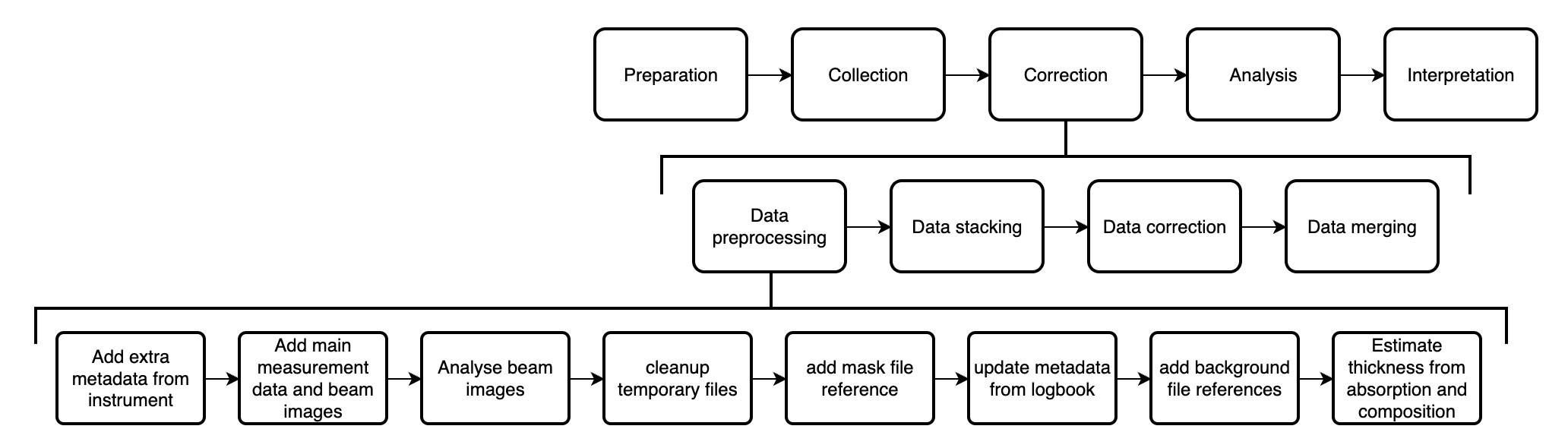
The data processing is done in several stages (Figure 2), with the preprocessing used to convert the datafiles into a NeXus-proximate format with all the necessary metadata in place for the subsequent steps. Measurements that were multiple repeats in the same configuration get stacked into a single file. After the data correction in DAWN, the corrected, now averaged data from each configuration gets merged (using our uncertainties-aware dataMerge code) into a single curve, and then we’re ready to go to the analysis.
The work so far
The preprocessing in the previous years consisted largely of a convoluted script called “structurize.py”, combined with a few auxiliary command-line programs. Maintainability of that code was terrible, so that needed to be changed rather than me trying to monkey-patch the code back to something halfway working.
The core of the new code is the HDF5Translator I wrote a while back, which forms a flexible way for translating data in any HDF5 structure into another structure, or even just doing input checking and unit conversions.
Since the preprocessing also consists of many other small steps, and requires metadata read from the logbook and the project/sample forms, I thought it wise to build a small pipeline manager program around that. The logbook and project/sample reading is handled by the logbook2mouse code, which also interprets sample compositions and calculates X-ray absorption coefficients and soon also scattering length densities. With the pipeline manager (which takes care of the bottom row shown in Figure 2), this externally supplied information only has to be read and validated once, and can then be used to process all the measurements without reloading. This simultaneously allows for some parallelisation in the data processing. Together with the code for the individual preprocessing steps, this pipeline is encapsulated in the MOUSEDataPipeline repository.
So… Where’s the rub?
After solving most of this robustness issues across the entire automated data processing pipeline (so it can tolerate missing or incomplete data as well), two issues remain. The first issue is that the new data quality is not fully up to my standards just yet. The second is that the absolute scaling may be less reliable.
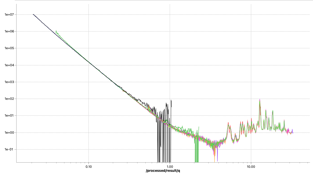
The first issue is that of data quality. Initially, the corrected data did not always line up nicely. That has been traced back to incorrect sample thickness determinations, and this is now largely resolved. Data now lines up again with scaling factors within a few percent of each other*. For a few weaker samples, however, there are still visible jumps where the data ranges from the different measurement configurations start or end. These seem minor, but to me they indicate trouble that even shows up for these easy, strongly scattering samples. This obviously incorrect data needs resolving before it negatively affects data we would analyse or publish. Let’s keep investigating where this issue comes from…
The second issue is that of absolute scaling. Samples with the same composition are too far removed from each other on the vertical axis for my taste. In the old MOUSE pipeline, these were matching much better. I will need to dive into the metadata and the metadata generation to discover what is causing this discrepancy. My initial suspicion is that it might have to do with the flux- and transmission measurements, or with the apparent thickness calculation.
Some investigation…
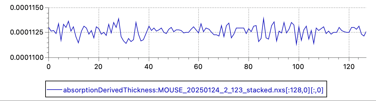
Since last Friday, we are running operando electrochemistry experiments on battery materials, and these experiments will allow me to eliminate a few possible causes and hone in on the actual problem. Initial results show a modest fluctuation of the automatically determined thicknesses (using the transmission factor and the x-ray absorption coefficient) with a standard deviation of about 0.5%. So transmission and thickness are probably not to blame.
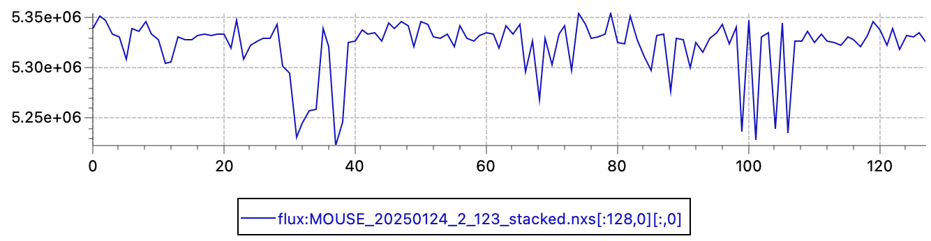
Primary beam flux shows a similar fluctuation (relative standard deviation of 0.53%, so a 95% confidence interval of about 2%). Given that the X-ray source is now running continuously for the last 8 years, I am not overly surprised by this fluctuation.
Both results do highlight that we would benefit from continuous flux monitoring to improve the data, perhaps with a back-fluorescing or a semitransparent beamstop of some sort. Here, we should remember the radiation hardening issues we had on the Anton Paar SAXSess, when combining a semitransparent beamstop with multilayer optics (see the ancient post here: https://lookingatnothing.com/index.php/archives/1949). Given those findings, we should understand that we can only use the intensity behind a semitransparent beamstop to be a measure proportional to the primary beam flux in these lab systems, and that this reading should not be used to determine transmission factors.
But I also remember that I modified the data processing pipeline sequence a little to accommodate the per-measurement, non-averaged thickness values. That places the background subtraction after the thickness correction, and that is not correct (also because the background will then be thickness-corrected with its own thickness). As we do not actually have changing sample thicknesses during the experiment, or at least not when comparing repetitions in a single, static experiment, the mean and standard error on the mean for the thickness should be calculated in a preprocessing step, and we can normalise the background subtracted, averaged data by that instead. After a bit more digging, I found a second miscalculation, using np.log10 instead of np.log (natural logarithm) in my calculation for the thickness.
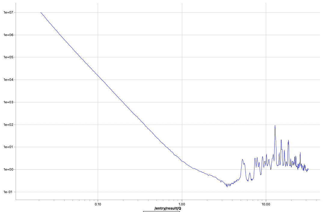
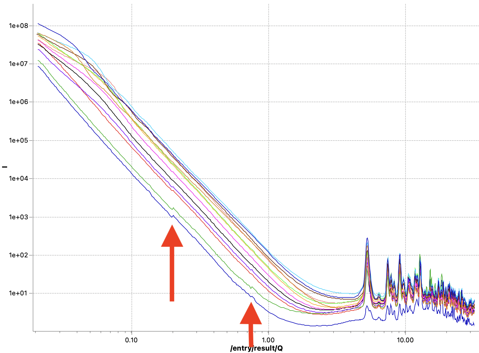
These two methods are now fixed, but did not completely solve the problems. I can now get rid of the little steps by switching off the autoscaling, as seen in Figure 6. That, combined with a miniscule difference in curve shape due to different beam sizes at the different instrument configuration settings (Figure 7), points me at another potential culprit: we will have to more closely match our collimations between the different ranges. Lastly, the worst offender shown in Figures 6 and 7 also has but a few crystallites in the beam, so that could be another cause for discrepancies between the ranges (as we illuminate more or fewer particles with different collimations). The hunt continues…
Conclusion for now:
It turns out that revamping a machine and a methodology that we fine-tuned over the course of seven years takes a bit of time. We also took the opportunity to change a few more things in the operation methods than we perhaps should have done simultaneously, making troubleshooting a bit harder. As the saying goes: “We don’t do this because it is easy, but because we thought it would be easy”.
But we’ll get there, step by step, and hopefully create a track that allows others to follow. While (with the latest changes) the data is now somewhat passable, it will be a few more months before our data is back to perfection. Until then, there’s lots of testing and calibration measurements to be done in between measurements.
*) strictly speaking we don’t need scaling factors as all our datasets are in absolute units. But, due to 1) variations in flux- and transmission factors between measurements, and 2) changing beam dimensions coupled with sample inhomogeneities, the scaling factors sometimes deviate a few percent. it should not be more than that, though.