

Our latest MOUSE collaborators, Ph.D. researcher Julia and Master’s student Keelin, are particularly excited about watching fat melt and resolidify. Not for a lack of reason: these particular fats are commonly used to make up margarine, and controlling the phase formation during the temperature cycling means controlling the way the margarine looks, feels, and tastes.
To control this phase formation in situ, we need 1) accurate temperature control, but also 2) the ability to rapidly heat and cool the samples. Rapid heating is no biggie (just add power), but rapid cooling is a more difficult challenge. To accommodate this temperature profile, we therefore built a set-up that can instantaneously switch between a hot and cold stream (see the previous post for the flow switcher details). Here’s how we integrated all that into a really cool experiment.

Why the fast cooling?
Now, I’m no expert on this topic, but Julia and Keelin tried their best to explain it to me. The idea is that, if you crash-cool liquid fats to different temperatures, these fats crystallise to different polymorphs. When we then gradually heat them up, they may then form another structure before melting. This means that by choosing particular temperature profiles in production, you can get your fats to be a little different. The crash-cooling also has a secondary effect in that it creates a great number of small crystallites rather than fewer larger crystallites.
In industrial processes, such fat (and fat mixtures) are crash-cooled in a scraped-surface heat exchanger: a cool-walled tube with rotating knives that scrapes crystallised materials off of the walls and mixes the crystals with other liquid phases present. This creates a composite structure, consisting of a network of small fat crystallites and globules, with an intermixed water phase.
In this study, we’re only looking at pure components, so life is a little easier for now (and we won’t expect anything significant at small angles for this reason either).
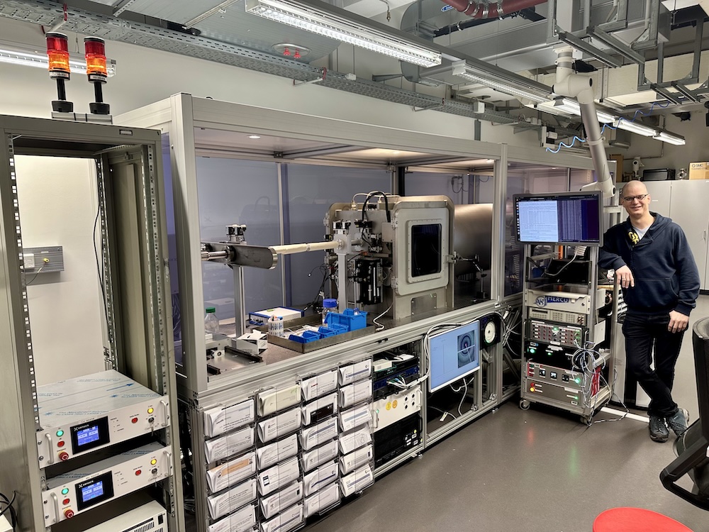
The Set-up and machine integration / automation
The good thing about this experiment is that we can melt and recrystallise the same sample over and over again. Secondly, as we are using temperatures of 80 degrees at most, we can use our favourite, noncrystalline Scotch Magic Tape, which also does not have a temperature-dependent scattering profile. Lastly, Julia and Keelin were only interested in a limited Q range, which means we could stick to one instrument configuration with the detector approximately 90mm from the sample.
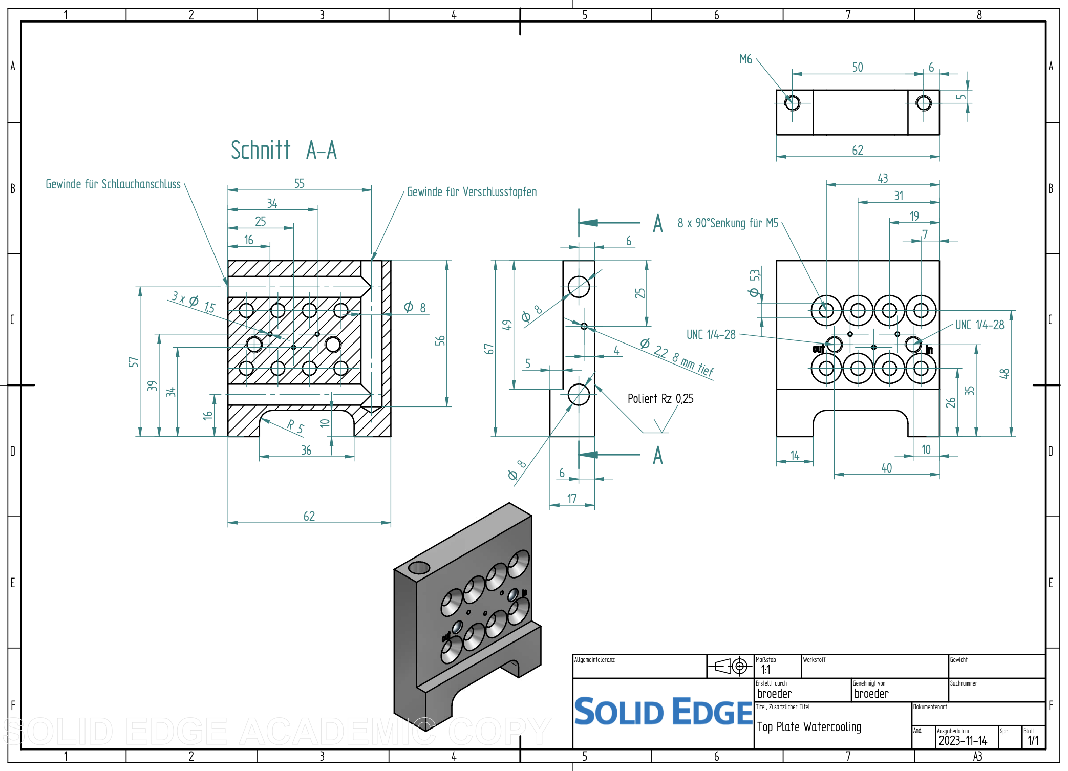
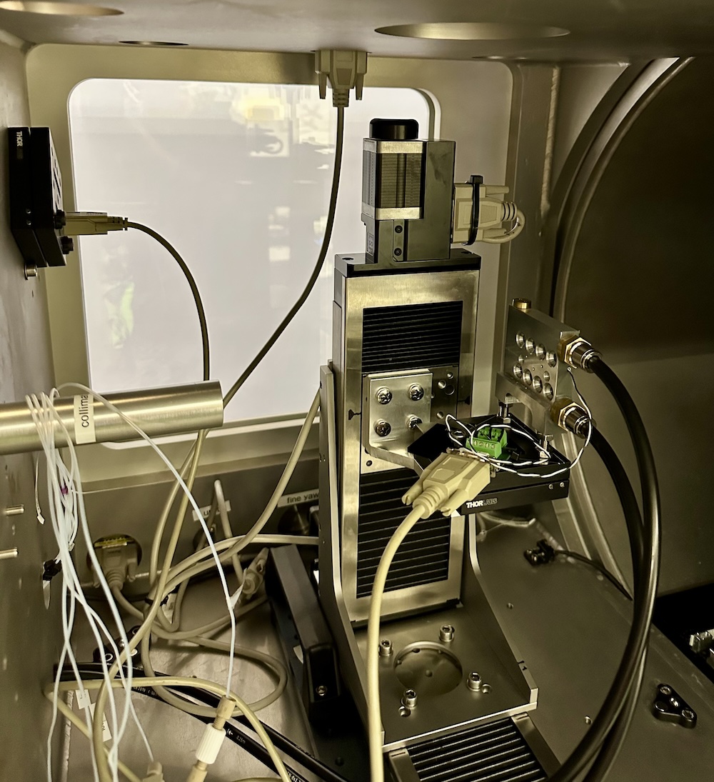
For this experiment, we used a modified version of this aluminium sample holder, which instead of a heating cartridge, has an 8 mm diameter liquid cooling channel following a U-bend around the sample positions (Figure 1). It offers three small sample positions of 1.5 mm diameter (deliberately kept small to ensure good heat transfer into the material). The sample thickness in the beam was about 1 mm, but with the bulging of the sample (and windows) in vacuum, the absorption-determined sample thickness ended up closer to 1.3-1.5 mm which was fine. We now also have a PT100 in the sample holder block, so that we can monitor something close to the actual sample temperature.
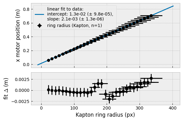
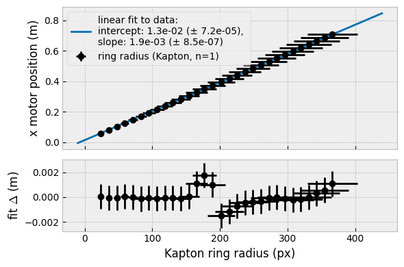
For propriety we also did a triangulation on the first-order fat ring of the crystallised samples (Figure 2, so we could get a more precise sample-detector distance (the original estimate was off by 1 mm).
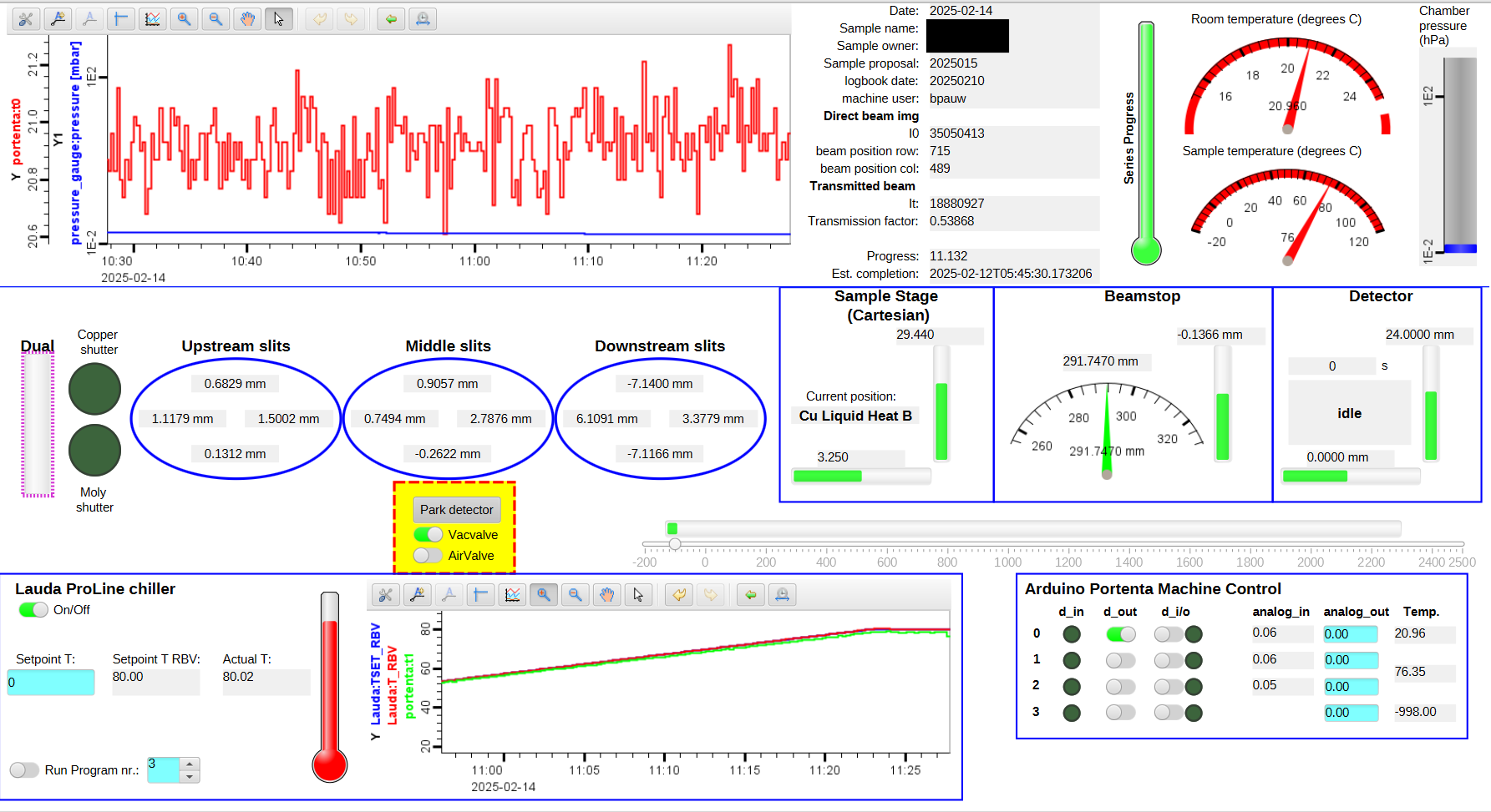
To get the desired temperature profile, we used two chillers, one small Julabo fixed at 80 degrees C, and a big Lauda for the lower temperatures and the accurate ramping. The latter is a good one for slow ramps, though this particular model with bath and external cycle (RP855C) is not manufactured anymore. To control this, I put together a quick EPICS IOC in a few hours to access the main functions: temperature setting and readout, start/stop, and start/stop of preprogrammed temperature profiles. These temperature profiles still have to be programmed on the chiller itself, but can be started by the IOC.
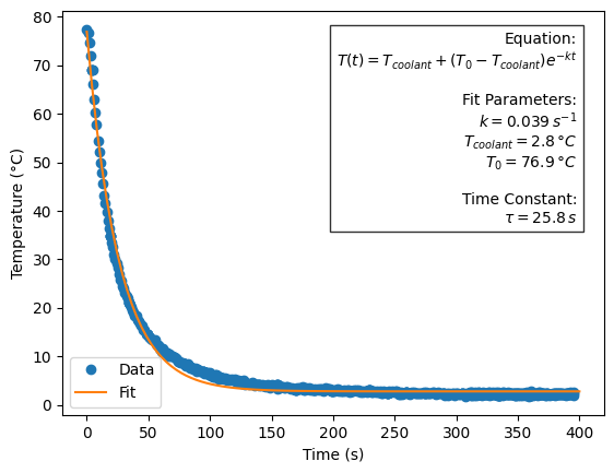
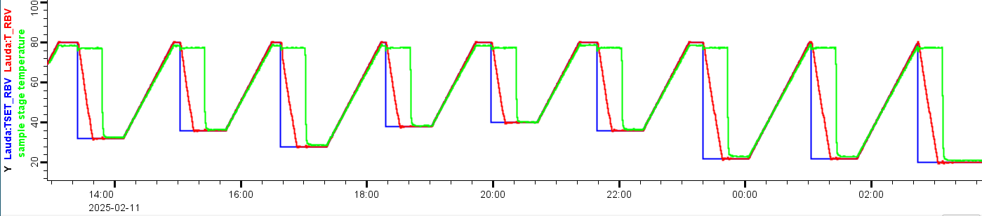
Lastly, we have the coolant flow switching device I talked about last time, to switch between the Julabo and the Lauda. This is needed to keep the sample at high temperature (molten) for a while, while the Lauda goes down to the desired isothermal temperature. When this then switches back to the Lauda flow, it’ll cool very fast, with about 80% of the temperature drop completed within 30 seconds (Figure 0). It could be sped up a bit more, but for now, this seems good enough. The coolant flow valves are driven by a 24V relay, which is controlled by our Arduino Pro PMC which outputs 24V by default. This Arduino is also used to read the (room and) sample temperatures every 15s.
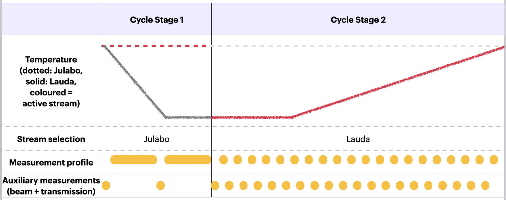
Now we get to the point where our large effort changing the control system is starting to pay off. We can now program complex orchestrations of our modular MOUSE components in Python to get the best possible data. The required two-stage orchestration for a single temperature cycling experiment is shown in Figure 3. In reality, we can get the temperature profile as shown in Figures 0 and 4.
The Initial Results…
During the experiments, the saturated triglycerides we’ve been investigating showed a variety of interesting structures. It will take a while to analyse the data and figure out what exactly has been going on, but for now, we’ve got some pretty videos of the changes. A sneak preview can be seen in Figure 6, which shows the formation of a lamellar phase (or at least the (001) and (003) reflections, the (002) reflection probably gets lost due to the convolution with the lamellar form factor being close to zero at that point, an assumption we need to verify). Secondly, the crystallite size appears to grow a bit towards the end, as evidenced by the slight narrowing of the reflections.

This dataset and the other (much cooler) ones will be further processed, analysed and cross-checked. Stay tuned and we will let you know once there’s papers with more in-depth analyses in the pipeline!
Thanks
Thanks to Julia and Keelin for bringing interesting experiments our way that pushed the boundaries of the instrument (and the instrument control). Thanks to Bettina at BAM for the technical drawings of the updated sample stage (sorry I haven’t had a chance to upload them yet), and thanks to Sergej for figuring out and assembling the coolant flow switch-over rig. Thanks to Ingo for his help with the server-side move to EPICS. Lastly, but not leastly, I’d like to thank Anja for her adaptations to the measurement scripting that helped transition the machine to EPICS and python for instrument control.