I’ve written a bit about MoDaCor in the past (in these and these posts, for example); building a framework to process our instruments’ data in a standardised, traceable manner. This is now getting to a stage where it’s producing some actual results, so I want to talk about the core software design and some of the early results.

Firstly, a disclaimer: I’m not a trained software architect, and so I’m likely to make some mistakes when it comes to nomenclature and diagramming.

The framework design

Organising modular operations in graphs

At the heart of the pipeline: a Processing Step

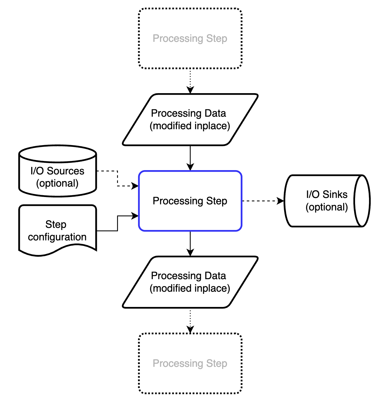
We want to process data in a modular fashion, so we can rearrange and modify the procedures at will. That means we need a fundamental “processing step” that we can wrap our maths in. This processing step should be called using exactly the same generic syntax, regardless of what it’s doing or where it is in the processing pipeline. The structure we ended up with is shown in Figure 1.

The processing step modifies a dictionary of processing data in place (see below). To do this, it may draw on information from the processing data itself, information from one or more io sources, and information from the step configuration.

To make subsequent executions of processing steps more efficient, each processing step can also store pre-processed data (calculated on first execution). This is helpful, for example, when calculating pixel coordinates in 3D or X-ray scattering geometries (e.g. Q, Psi, TwoTheta, Omega/solid angle matrices). The first execution of the process step can store these objects in an internal cache after calculation, and assign the links to subsequent DataBundles that pass through it. That changes the execution time (of this unoptimised processstep) on my laptop from about 0.7s to about 0.0001s.

Besides outputting the modified (or augmented) processing data, ready for the next processing step, it can also dump some information into an io sink (= direct output). Lastly, the processing step contains internal documentation describing what it needs and what it does, some of which is validated, and other parts which may be useful later for graphical pipeline configuration tools.

The Pipeline

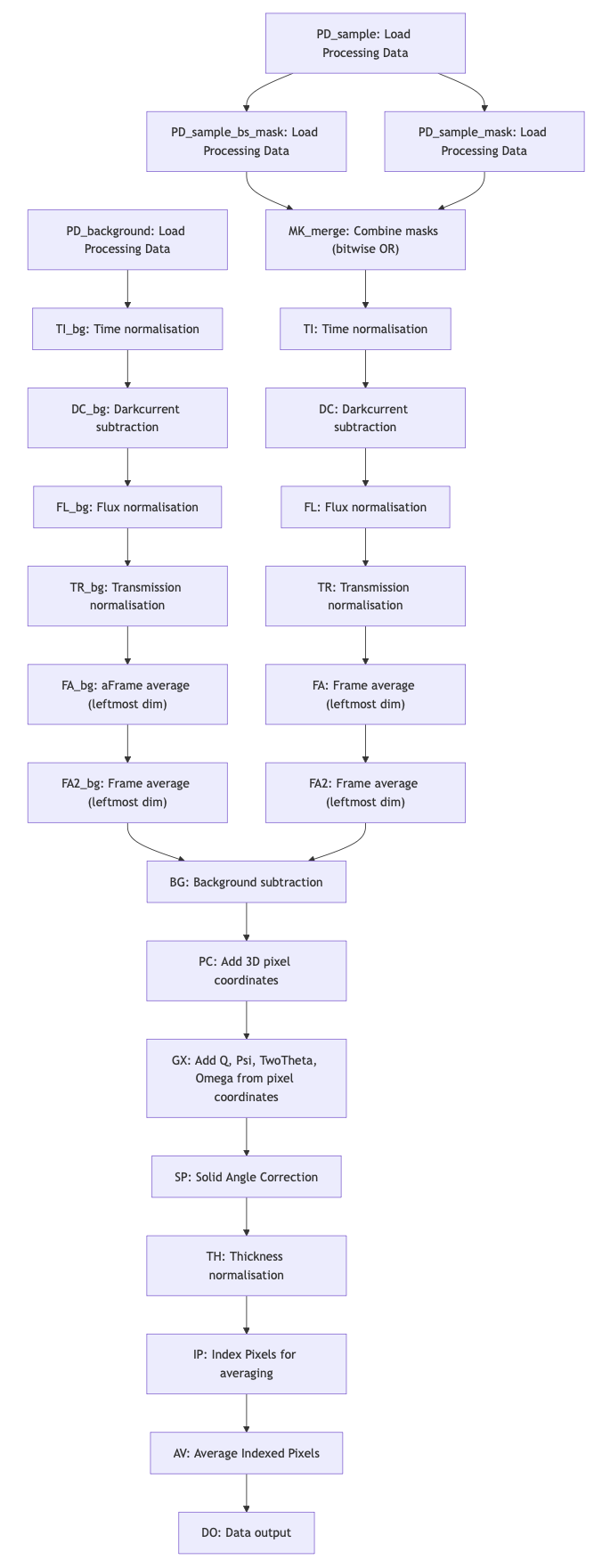
The processing pipeline allows us to program and organise the processing steps in the right sequence. Graphs are ideal for this (c.f. Figure 2, or this link). Since we may need to process data in several pipelines before combining them, our graphs support both merging as well as splitting branches.

Consider, for example, that you get data streamed from an instrument. You want to do some basic processing on this data, after which you will send it to a live data viewer. At the same time, you want your data to also be processed thoroughly and stored as files (or as subsequent frames in the same file) or uploaded to a database.

Splitting branches can be useful for cases such as liquids in capillaries, where you want to have two variants of your data: one where just the capillary background is subtracted, and another where also the dispersant is subtracted. Then you can address issues like these at a later stage.

The pipeline in Figure 2 is automatically constructed; we indicate in the pipeline configuration file (a YAML file) for each processing step, which other processing step(s) it relies on. The topmost processing steps have no dependencies, and nothing relies on the final step. That means that we can reorganise or merge branches simply by indicating the dependencies. Each processing step is then executed in sequence based on its position in the pipeline.

For branching pipelines, we will have to make a separate processing step which duplicates a DataBundle. The branch can then operate on the copy rather than the original, so both are now independent. This has not been implemented yet.

As you can imagine, debugging such a modular pipeline is not easy. You can pause the execution at any point and inspect the state of the ProcessingData dictionary, but that gets tedious very fast. Fortunately, we’ve implemented a pipeline tracer, that follows and records the mutations of selected DataBundles at every processing step, highlights changes to units, shapes and uncertainties, and keeps track of timing (for future profiling). This is very helpful for debugging and tracing. For example, a part of such a trace summary might look like this (with purple squares indicating a change occurred, and green squares indicating no change):

Step DC_bg — SubtractBySourceData — Subtract by IoSource data ⏱ 79.15 ms

Step TI — DivideBySourceData — Divide by IoSource data ⏱ 95.47 ms
└─ • sample.signal [dimensionality, units]
    🟪 units              count/px → count/px/s
    🟪 dimensionality     1 / [detector_pixel] → 1 / [detector_pixel] / [time]
    🟩 shape              (16, 1, 1065, 1030)
    🟩 NaN(signal)        0
    uncertainties:
      🟩 NaN(unc['poisson']) 0

Step FL_bg — DivideBySourceData — Divide by IoSource data ⏱ 107.41 ms

...

Step FA — ReduceDimensionality — average or sum, weighted or unweighted, over axes ⏱ 45.45 ms
└─ • sample.signal [shape]
    🟩 units              1/px
    🟩 dimensionality     1 / [detector_pixel]
    🟪 shape              (16, 1, 1065, 1030) → (1, 1065, 1030)
    🟩 NaN(signal)        0
    uncertainties:
      🟩 NaN(unc['poisson']) 0

This makes tracking changes in units, shapes and NaNs much easier. The full trace of the pipeline run is stored alongside the pipeline configuration and module documentation in a (gigantic, very information-rich) JSON structure for future inspection.

Naturally, future users will not want to code YAML configuration files by hand or inspect traces. A (web-based) user interface such as React Flow will eventually be needed to make pipeline configuration accessible and debugging easier. For this, the pipeline module also allows pipeline export and import from dot and spec formats, and easy visualisation using mermaid in jupyter notebooks is already heavily used (Figure 2 was made using the online mermaid editor based on the output of the MoDaCor pipeline).

So far, the pipeline reads configurations, executes the modules in sequence, and the trace is populated. The pipeline can be reset for the next sample data and re-run, which will exploit the cached pre-calculated information on the second execution to bring down execution times.

While we haven’t spent any effort yet on speeding up computation, on my MacBook Pro M1, the pipeline in Figure 2 applied to a (16, 1, 1065, 1030)-sized stack of frames takes 2.6s on the first run, and 1.3s on the second. But let’s take a look at what it does to the data, by delving into the information carriers next.

The foundational information carriers

BaseData: the foundational information carrier

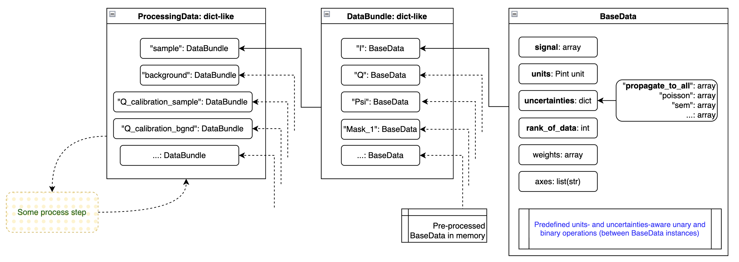
The most basic information element that we are working with is the BaseData element (Figure 3, right-hand side). This can carry an arbitrarily large array (also single-element arrays for scalars). It contains the basic pieces of information necessary:

1. the signal of the data
2. the units (as a Pint unit)
3. the uncertainties (a dictionary of uncertainty estimators, e.g. a Poisson / counting statistics estimate and a standard error on the mean estimate, or a propagate_to_all uncertainty estimate)
4. the rank of the data (RoD), useful when loading a stack of frames of (16, 1, 1065, 1030), where rank_of_data=2 would indicate that only the last two dimensions are the data dimensions, the rest is excess dimensions
5. axes, so far unused, but akin to the NeXus definition of axes, allowing to indicate what each signal dimension is supposed to mean.

BaseData also contains the logic for handling units, uncertainties and array broadcasting when operating with itself (unary operations) or operating with other BaseData instances (binary operations). One peculiarity here is the handling of the multiple uncertainties, which follow the deterministic rules explained here. Units are matched (if needed and if possible) before operations, so you can happily multiply a quantity in imperial milli-yards with one using megameter.

This greatly simplifies the processing step modules: as long as each piece of numerical information is translated into a BaseData element, you can do normal maths operations knowing that everything is kept consistent under the hood. Any inconsistency occurring during the operation will be raised to the user. Practically, that means that you need to explicitly specify a lot of the previously assumed units, e.g. darkcurrent has units of counts/pixel/s, and a certain propagate_to_all uncertainty estimate, that will be mixed in and propagated with the other uncertainties. This also means that if you are unhappy with the way uncertainties are handled, this is the central location where you can adjust its behaviour for all processing steps.

DataBundle: Binding BaseData together that belong together

The DataBundle bundles BaseData instances together (as implied by the name). For example, I have a DataBundle that belongs to my sample measurement. This contains BaseData instances such as ‘signal’ (a.k.a. Intensity), ‘Q’, ‘Psi’, ‘mask’, ‘beamstop_mask’, ‘Omega’ (solid angle), and many more. They all belong to the same dataset though.

Some processing steps, such as those calculating pixel coordinates, can create extra arrays. As mentioned before, these same python objects can be added to multiple DataBundles at no extra computational cost.

ProcessingData: All the DataBundles needed for a process

There’s one more level, mostly just an administrative one. We want to feed one data carrier to each processing step, regardless of how many DataBundles we may be working with. So the ProcessingData dictionary is a collection of different DataBundles. For example, I may have the following DataBundles in ProcessingData: ‘sample’, ‘background’, ‘Q_calibration_sample’ (e.g. silver behenate or some NIST diffraction standard), ‘I_calibration_sample’, and any other bundle that might be relevant for processing this sample.

IoSources: where data originates

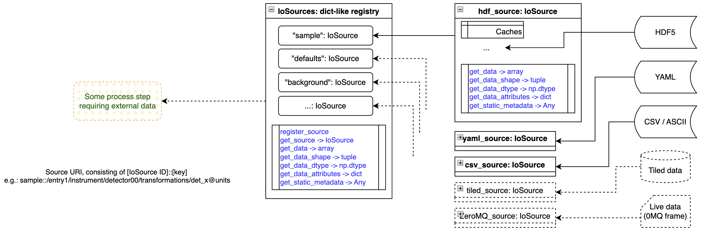
Whatever we do, we’re interacting with experimental data. This data has to come from somewhere, though we may have many diverse sources in an experiment. We may have default values coded in a YAML settings file, reference data in a CSV file, background measurements in HDF5 format, and live sample data coming in over ZeroMQ or via Tiled.

We need a consistent, source-agnostic manner of accessing this data. While I initially wanted to avoid this altogether and use Tiled directly, using it in a user environment (read: some poor student’s laptop) may be not easy nor performant. Therefore, we came up with a format that is very close to Tiled (and inherently compatible with it), yet allows us to have our own data loaders for more lightweight implementations.

Our loaders (IoSource instances) can also cache data, improving performance on repeated use of the same data. They only have a handful of methods to read numerical and non-numerical (meta)data, and don’t do anything special. For loading partial data (lazy loading of large arrays, for example, to be processed in more manageable chunks), you can also forward a slice object to the data load method, though this is untested as of yet.

The IoSources registry is nothing special again, but, like ProcessingData, is combing the various sources into a single object. That allows us to access any source using a single method in IoSources.

IoSinks and the individual IoSink instances work exactly the same but for outputting data as opposed to loading data.

Getting wild… SAXSess data

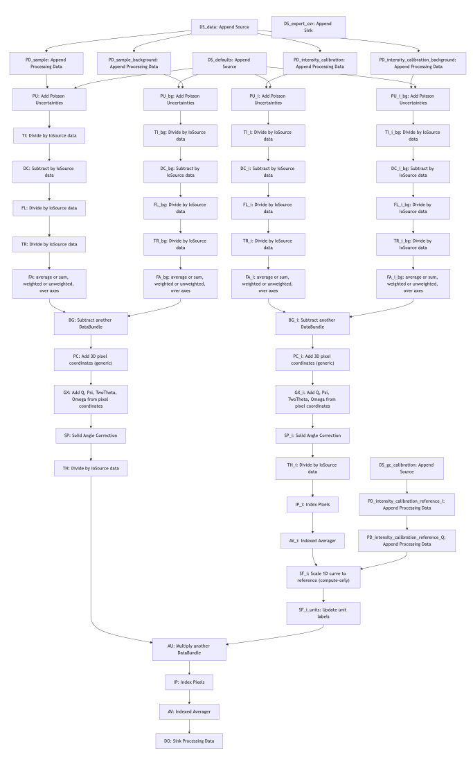
So for our line-collimated SAXSess data we have developed a pipeline as well (Figure 5), that is similar but a bit more extensive than the MOUSE pipeline shown in Figure 2. When you look at the general structure of the pipeline, you can see two instances of the “two paths merging to one” path, and with some more bits and bobs attached to it.

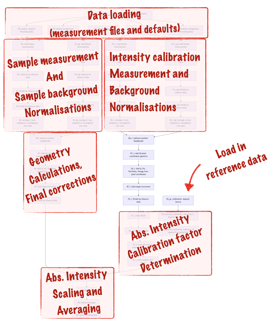
To explain the added complication, I’ve outlined the different sections in Figure 6. The extra fork on the right-hand side is for the glassy carbon intensity calibration measurements, which we use for scaling the sample intensity (calculated in the left fork) to absolute units. Other than that, it’s pretty much the same pipeline.

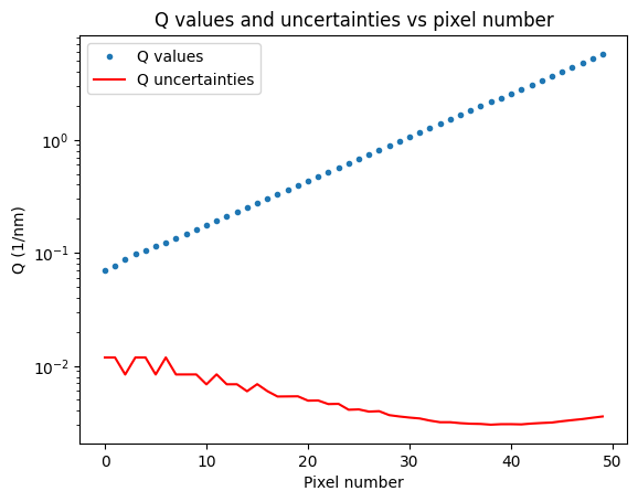
The end result of this is that we now have datapoints with both horizontal and vertical uncertainties. At the moment, I only have one of four intensity uncertainty components shown, and only one of two Q uncertainty components, a future processing step will combine the different uncertainty estimates. We can, however, see that the Q uncertainty is Q-dependent (as we saw when we derived this for the MOUSE Q uncertainties), this is more clearly shown in Figure 8. This means that the resulting uncertainty on sizes determined with this instrument, is also dependent on how large the particles are (which defines where they scatter, and therefore what their Q uncertainty is).

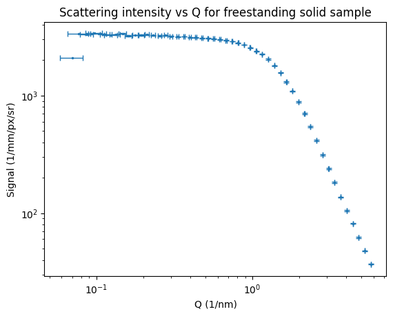
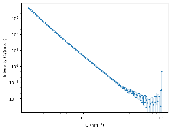
For the most boring sample in the MOUSE instrument that I used for testing (sorry about that), we also can see some 1D data coming out. As the input uncertainties for each machine parameter are not yet correctly set, the output Q uncertainties are not very informative. Updates to follow on this in the future, for now I just wanted to show that the thing is producing some useful output.

What’s next?

Next up, I will work on completing the two use cases for us, that means working on combining uncertainty estimates and completing the last few missing processing steps. From that point on, it’s time to publish on the approach, and work towards exploiting this as a reference data processing procedure.

Thanks to the international MoDaCor team with whom we got the foundation started in the code camp from last May, who brought valuable input and insights from many viewpoints. I hope this work will be useful to many more people in the future.