

[A note because I cannot stand being imprecise in terminology: what is commonly called “Solvent” in scattering, is better expressed as: the dispersant medium, i.e. the medium that disperses your analyte. This can be liquid, solid or gaseous… I haven’t seen plasmas used for this yet.]
We’ve all heard about the infamous “hydration shell” that (at least ostensibly) surrounds proteins in solution: a shell of solvent molecules that orients to, and surrounds the protein. This shell scatters differently than the bulk solvent, and needs to be taken into account in the model. Try to subtract it, and you end up with incorrect subtraction of the assumed background signal. It turns out this is not just limited to Bio-SAXS, but can happen to anyone measuring dispersions. So what can we do about it?
Even in our laboratory, we occasionally see hints of interactions of the analyte with the dispersant medium. After all the corrections have been done, and the displaced volume correction accounted for, this can lead to an incorrect, negative signal, indicative of an oversubtraction of our assumed background signal.
One example is shown in Figure 1. Here, we are trying to isolate the signal from a small molecule in a dispersant, but when we focus on the subtracted (dark grey) data in the wide-angle region, we see a place at around Q=18 1/nm, where there is evidence of an oversubtraction. We are keeping as much as possible the same, using the same flow-through capillary in the same location, and doing the entire universal data correction chain with decent, precise metadata.
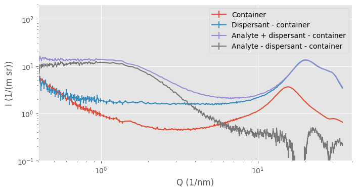
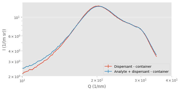
What happens is that our assumption no longer holds: the assumption that, outside of the analyte, the background is a homogeneous, noninteracting block of material. If our dispersant changes in structure due to the presence of the analyte, the “background” signal changes, and we can no longer justify subtracting the non-identical signals. For example, when we zoom in into the region where we see the “amorphous halo” caused by our intermolecular distances, we can detect the tiniest of differences in the solvent signal (Figure 2). This shows that the dispersant structure is somewhat affected by the presence of the analyte. If we were over- or undersubtracting, the entire curve would be shifted without a change in shape.
What do we do now?
Practically, this means that we usually calculate two signals for samples dispersed in liquids for our users: one with the capillary and dispersant subtracted, and one where we only subtract the capillary. The latter is usually the more authoritative, but it is now hard to identify any sample signals amongst the relatively massive signal of the dispersant (Figure 1).
Since we want to do things absolutely correct, we will also not consider “fixes” that would subtract variable amounts of background. This includes methods such as “subtracting just enough background until you are just shy of getting negative intensity values”, because you don’t know what the scattering level at that minimum point *should* be.
Additionally, since your analyte is actually changing the structure of the dispersant, the scattering signal of the dispersant is no longer identical. It is different from that which you recorded during your background measurement, and therefore no longer valid for the sample. Apropos, this is why you should measure your dispersant with as many of the components (buffers, salts) as you need to most closely approximate the signal of the dispersant with your analyte in.
The open question remains now about which data is better for us to work with. The data with the background signal removed and possible negative intensities (to be accounted for in the scattering model as the difference in dispersant structure), or the data with the dispersant in place?
The case for keeping the dispersant signal in the scattering signal
The latter option, i.e. not subtracting the dispersant at all but only the container, would definitely be easier from a data analysis point of view. You can model your background signal in the same way you would model the analyte signal.
I have been impressed by one student, who carefully modelled their background in addition to their analyte signal for an in-situ (flow-through) measurement of a reactant mixture. They calculated remaining component concentrations in the dispersant based on the reaction coordinate and the signals from the individual components to construct the dispersant signal. This is definitely the right way of doing this. Similarly, if you understand your dispersant behaviour well enough, you might be able to approximate the effect of structural changes due to the analyte presence to the dispersant signal.
The downside is that the signal of the analyte in relation to the dispersant will now be minuscule, and any hopes of visually recognising analyte signal features in the plotted data are now lost. You will need tricks such as (relative) difference plots to fish these out again and make them visible. There is one visual upside: the data, especially at intermediate Q does not look as noisy..
The case for subtracting an incorrect-but-close dispersant signal
If we accept a slightly larger possible uncertainty on the dispersant signal to account for the variations due to analyse-induced structural changes, we could subtract it and extract our analyte signal. That analyte signal will have larger uncertainties in certain areas where the behaviour of the dispersant signal is less well known, but hopefully we will see some significance nonetheless. (This does mean that we should measure our dispersant under a variety of conditions to find out where and how it might change.)
If we do this, we now have the advantage of using simpler analytical models for our data fitting, focusing only on the object of interest, largely cutting out anything that is of no interest. It is also the historical way of treating SAXS data, leading to less resistance on the path to publication, and for non-interacting systems it remains a perfectly valid approach. This signal also allows for much easier visual inspection and identification of features and changes, which, if you have trained your reciprocal eye, can be very helpful.
So which one…
Personally, I am torn on this, but I think we should treat it the same as we do for smearing effects: use one way for visualisation, the other for data analysis. Which brings me neatly to my next point: we definitely need to update our default visualisations.
To be continued…