

Just a couple of housekeeping notes: I’m giving talks in Europe in a month at the following locations:
- Unité Matériaux et Transformations (UMET), Lille on May 16, hosted by Grégory Stoclet,
- Birmingham University, Birmingham on the 20th of May, hosted by Zoe Schnepp,
- Nottingham University, Nottingham, on the 23rd of May, hosted by Philip Moriarty,
Between these dates, I’ll also be joining Zoe and Martin for beamtime at the Diamond synchrotron (beamline I11) between May 21 and May 23. Please feel free to stop me at these locations and say hi!
For today, I’ve got another bit of data correction to show. I thought it might be interesting to put them all together and show you what difference it makes to an integrated scattering pattern. Many of the data corrections implemented are quite straightforward shifts and scalings, but some are more involved and have a greater effect on the scattering pattern. First, let’s put all of them out there. This data is a sample of MgZn alloy, in early stages of precipitation. It has been measured for three hours on a reasonably good Bruker instrument with a low background (all-vacuum flight path, good collimation), and a Bruker HiStar wire detector which I have complained about before. The new high speed molybdenum rotating anode source is quite stable (varying about 5% in intensity over the weeks I have been using it) and hasn’t let me down yet unlike a particular (older) Rigaku generator which is starting to make funny noises *again*. Anyway, I digress…
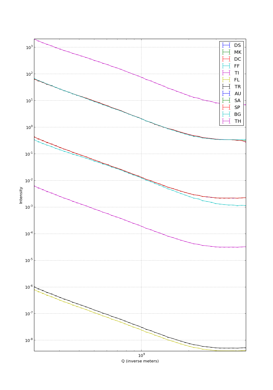
Figure 1 shows the collected data through its various correction steps (click on the image to enlarge). It is obvious that there is a lot of scaling going on, but there are also a few corrections that change the measured profile.
The corrections performed are (in this order): DS, DC, MK, FF, TI, FL, TR, AU, SP, SA, BG, TH (abbreviations are in this paper, software here. The correction abbreviations used here mean (respectively): data read-in, darkcurrent, mask, flatfield, time, flux, transmission, absolute intensity scaling, spherical (area dilation), self-absorption, background and thickness). GD (geometric distortion) is performed by the Bruker software. PO (polarisation) is still missing, as is MS and SM, DT and GA (multiple scattering, smearing effects, deadtime and nonlinearity). I don’t expect these to have large effects, but seeing is believing.
The biggest changes here happen for BG, making it particularly important to get right. Smaller changes are seen for MK (especially for the last few datapoints) and FF (raising and lowering particular datapoints by about 5%).
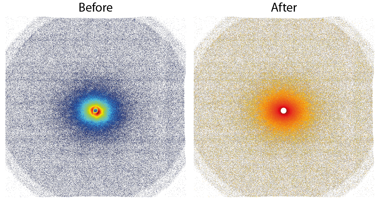
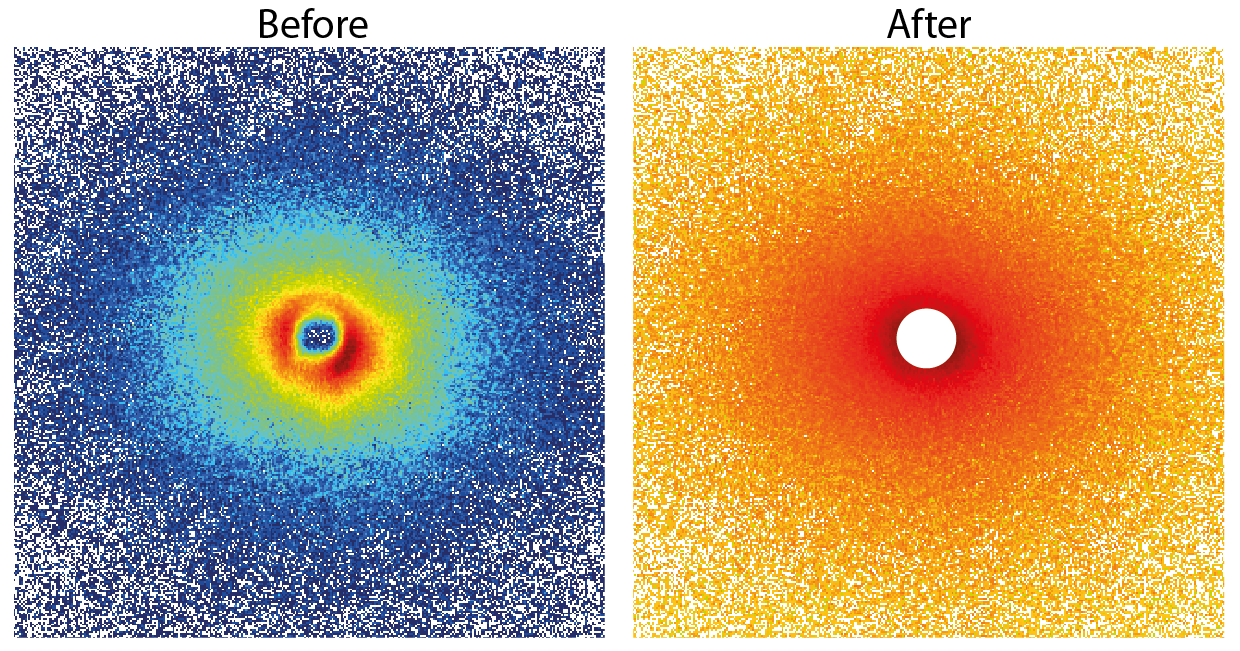
When comparing the 2D images rather than the integrated data, we see that there are a lot of changes occurring in the patterns upon correction (Figure 2, click to enlarge). We are expecting a little anisotropicity in this sample (which is visible). I hope it is clear from the differences before and after correction, though, that we have been able to successfully remove most of the “shit”. Just to drive home the point, Figure 3 shows a close-up of the central part.
In conclusion, data corrections are an essential but typically underrepresented part of small-angle scattering. It’s critical to get your data right, because all your conclusions will depend on it!
Leave a Reply