

[ed: My current project is running at an end, so if you happen to have a job offer I cannot refuse, I will seriously weigh it against the (tenured) job offer I got from NIMS!]
The typical argument in favor of the line-collimated “Kratky”-type instruments is that its X-ray flux is very high and that therefore you need only short measurement times. However, its data needs to be corrected through a “desmearing”-procedure, amplifying uncertainties and noise in the process. Does this approach then really give you better data? Let’s find out!
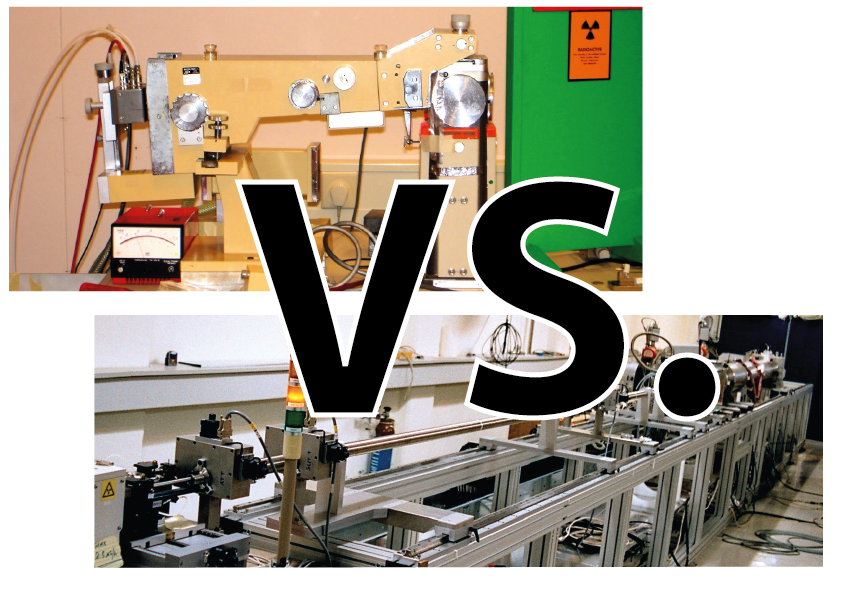
The instruments available for this comparison were an Anton Paar SAXSess system and a Bruker Nanostar. These are common instruments, but have one major difference: the SAXSess is a line-collimated “Kratky” instrument, the Nanostar is a pinhole-collimated system. Note that I am not interested here in comparing the manufacturers at all, but rather the underlying concepts.
The sample chosen for this is one of the glassy carbon standards produced by Jan Ilavsky, which comes complete with its own calibrated datacurve to compare against. The sample was measured for 10 minutes on both instruments (which was considered long enough by the Anton Paar representative who happened to visit).
Caveats: both instruments suffered from a drawback complicating direct comparisons; the SAXSess is on a tube source whereas the Nanostar is on a rotating anode generator. On the other hand, the SAXSess uses a nice sensitive and accurate Dectris Mythen detector, whereas the Nanostar is using an inefficient (at the used energy) gas-filled wire detector. So it is not a perfect comparison, but we make do with what we have.
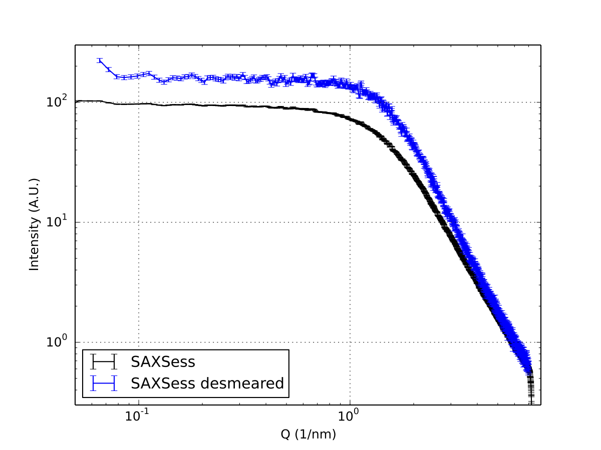
Andreas Thünemann kindly measured the sample using the Anton Paar instrument and corrected the data according to their recommended procedures. Before desmearing, the data looks to be of beautiful quality: low noise and small error bars (black curve, Figure 1). After desmearing, however, the uncertainties are much larger, and there is a visible structure in the data which is not expected for glassy carbon samples.
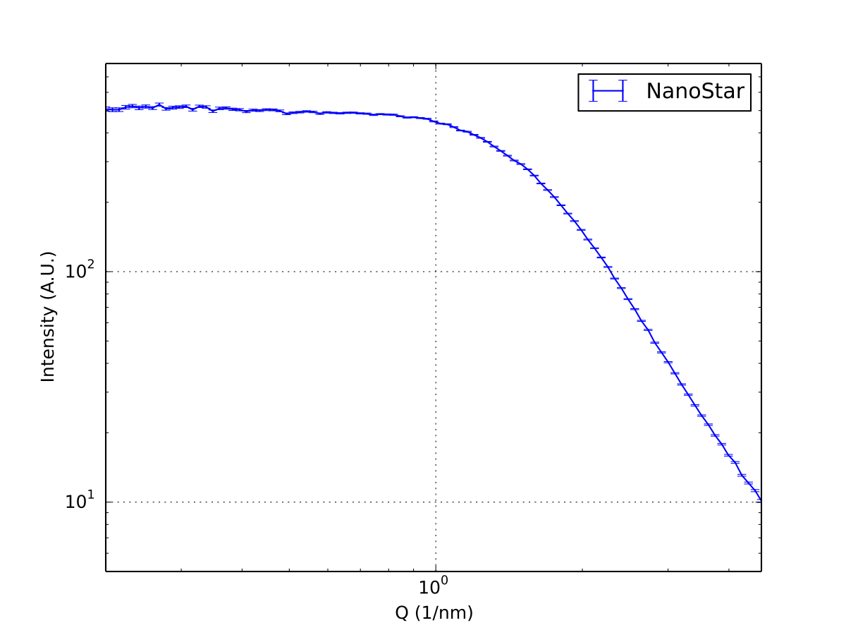
The Nanostar data (Figure 2) does not need desmearing (though it can be considered), but it has been heavily corrected using the in-house developed imp2 correction software. The data shown shows the smaller measurement range of the instrument (mostly because of the relatively poor detector performance), and shows a generally consistent scattering profile without outstanding features beyond the uncertainties.
So, how can we compare these datasets accurately to the calibrated curve supplied by Jan Ilavsky? First of all, the SAXSess data was binned to 100 logarithmically-spaced datapoints, in line with the bins from the Nanostar data correction procedure. The curves were then matched to the calibration datacurve using an error-weighted least-squares fitting procedure also allowing for a flat background contribution. The relative difference was then calculated for comparison.
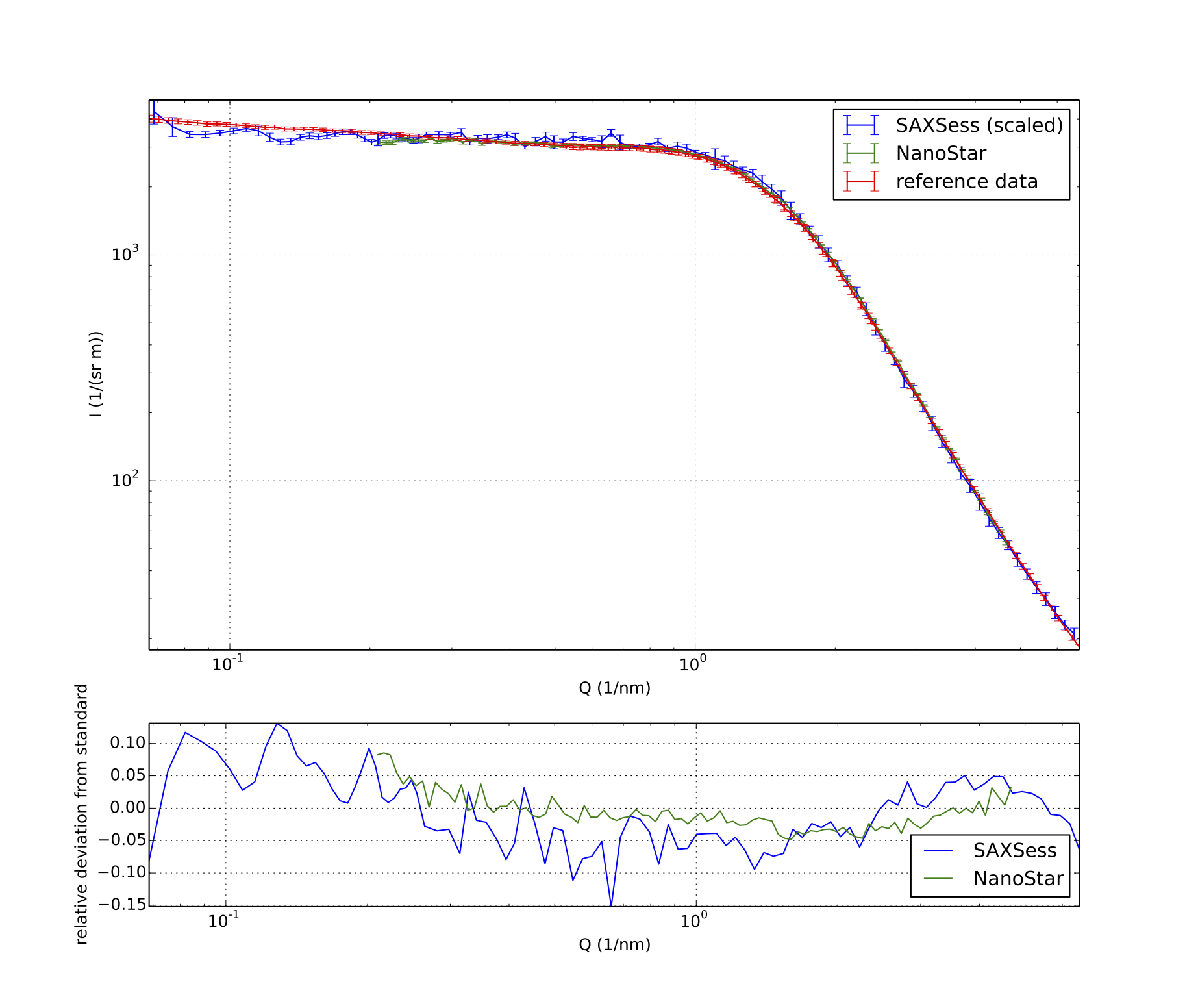
The results are quite informative (Figure 3). Mostly, the oscillations of the (blue) SAXSess scattering are more pronounced when directly compared with the (red) calibration data. The (green) Nanostar data, however, does deviate noticeably from the calibration data at low Q, which convinces me to re-check my data corrections.
The relative deviation plot, though, shows the real answer to the posed question. The required desmearing procedure applied to the SAXSess data negates any benefit there may have been of the increased photon flux. The data subsequently suffers from deviations in intensity in excess of +/- 10%. The Nanostar data shows better consistency with the calibrated data of +/- 5%, though that is not as good as I had hoped it would be.
In conclusion, then, please take care to measure on line-collimated instruments for a longer time. Try to compare the data of calibration samples to estimate the data uncertainty and be careful to optimize the desmearing procedure to minimize the resulting error magnification. As usual, comments can be posted below!
To me, the biggest issue by far with Kratky cameras is the danger of entirely overlooking features. In particular in Soft Matter, one often measures scatterers near Zero Average Contrast conditions (e.g. most micelles, with an excess electronic density in the shell), leading to a sharp minimum (inversion of the sign of the form factor amplitude at mid q). This sharp minimum can be completely missed with a Kratky camera, the de-smearing procedure providing a spectrum with a plateau at mid q that can be understood as due to repulsive interaction. Such an example exists in the literature with DPC micelles, and it is instructive to compare the synchrotron data from APS (Lipfert et al. DOI:10.1110/ps.051874706) to SAXSess data (Glatter et al. DOI:10.1021/jp9114089). In log scale, the difference is striking.