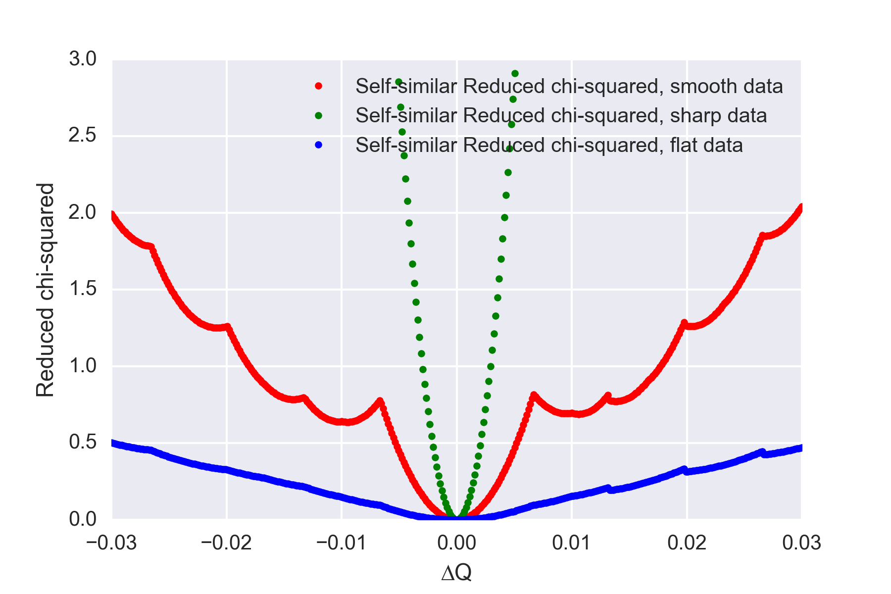
The evolution of the reduced Chi-squared as a function of the shift along q.
A funny point came up last week when we were trying to assess the Q-uncertainty inherent in our measurement. We were trying a method inspired by one from Christian Gollwitzer (part 3.3.2, paper here). What we did is the following:
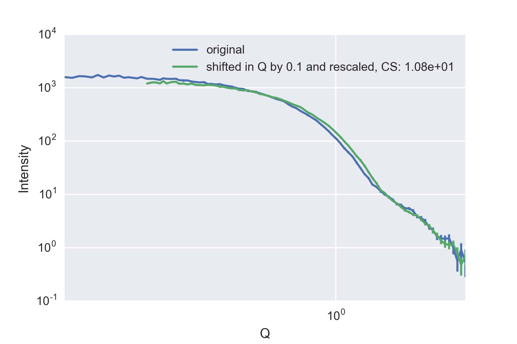
Figure 1: A pattern with sharp features compared to itself shifted by 0.1 1/nm.
We take a given measured pattern (absolute scale, complete with uncertainties), and shift it by a tiny bit in . We then compare the fit of the shifted pattern with its original (including scaling the intensity), and calculate the goodness-of-fit parameter (Figure 1). In order to calculate this self-similar , we do need to perform a (linear) interpolation on the intensity and the uncertainties.
Figure 2: A smoothly decaying pattern compared to itself shifted by 0.1 1/nm.
With this method, we can calculate the dependency of for a given shift in . As you may remember, when the two patterns overlap on average to within the uncertainty of the data. The shift at which we reach is our maximum allowed shift (Figure 4).
Figure 3: A mostly flat pattern compared to itself shifted by 0.1 1/nm.
This maximum allowed shift will vary depending on the shape in the datasets: the allowed is small (0.005) for patterns with sharp features (Figure 1), broader (0.04) for smooth patterns (Figure 2), and very large (0.1) for flat profiles (Figure 3). These values should be compared with the smallest q value in our data: . So what we seem to have, then, is some sort of measure for the -dependent information content in the scattering pattern.
Figure 4: The evolution of the reduced Chi-squared as a function of the shift along q.
This could maybe be used to estimate the uncertainty in our -vector, provided we take a pattern with sharp features, and preferably know the size of the object that it represents. Perhaps something silver behenate would do. In any case, we know that the uncertainty determined in this manner lies well below the width the datapoints themselves describe.
For now, at least, we have an interesting measure and some food for thought.
1 Comment
The uncertainty in the q-vector is an important measure. But a priori it is not clear how it affects the parameter of our, let’s say, fitted model. For large spheres of low dispersity, a shift of the q-vector has a dramatic effect. But if you measure the absolute intensity of water, i.e. its isothermal compressibiliy, a huge shift of the q-vector has no effect. Therefore, I think that it is important to know what you are looking at to estimate the uncertainty of your parameteres.


The uncertainty in the q-vector is an important measure. But a priori it is not clear how it affects the parameter of our, let’s say, fitted model. For large spheres of low dispersity, a shift of the q-vector has a dramatic effect. But if you measure the absolute intensity of water, i.e. its isothermal compressibiliy, a huge shift of the q-vector has no effect. Therefore, I think that it is important to know what you are looking at to estimate the uncertainty of your parameteres.