Now you see me, now you don’t: detectability in SAXS

Detectability of your analyte in scattering experiments, i.e. whether or not you can detect the scattering from the bit of your sample that you’re interested in, isn’t always easy to predict. But we can predict something, so that you can discover whether your experiment is worth trying before putting the fire to the iron. This saves time and lets you manage the expectations of your fellow materials scientists who were looking to apply that one amazing technique everyone is talking about to their material.

For this explanation, I will assume you have an instrument with a good, photon-counting detector (and bypass the discussions about the effects of CCDs, FReLoN detectors or image plates on the detectability). Additionally, I will use the following terms:

• Analyte: That part of the sample you want to characterize. This can be as simple as nanoparticles or micelles, but it can also mean the pores in a porous material, or precipitates in an alloy.
• Dispersant: The stuff your analyte is dispersed in (and surrounded by). In case of liquid dispersions, this is the solvent or suspending material, be it your water, buffer, or hexane. In metal alloys, this is the bulk material, in powders, this is the surrounding air. In essence, the dispersant is what holds your nanostructure in place.
• Container: The thing that contains your sample in the beam. This can be a liquid cell, a capillary, or two pieces of sticky tape. In case of freestanding materials such as foils or discs, the container doesn’t exist from a SAXS perspective, and we have one less background contributor to worry about.

So, back to the question of detectability. To understand why it is so complex to figure out, we need to look at the interplay of everything that affects the detectability of your samples:

Firstly, let’s talk about contrast: If your analyte has a scattering cross section (roughly proportional to the electron density) as large as the dispersant, you’ll not see it at all. Just as with contrast in TEM and photography, the material you want to look at should look and scatter differently than its surroundings.

Contrast

In general, however, the larger the contrast, the better the detectability. Gold nanoparticles dispersed in water scatter very well, silica reasonably well, and polystyrene in water scatters preciously little. With proteins, it’s a bit dependent on the type and conformation of the protein in the dispersant, so YMMV.

This can be a problem with some liquid dispersions, as materials often disperse most stably in liquids of roughly the same density. This issue can be (partially) avoided by adding a stabilizer to your analyte, which surround the analyte and make it compatible with other dispersants. With nanoparticles such as silver and gold, this can be achieved by coating them with a polymer stabilizer to help them disperse better (and longer) in liquids. Alternatively, you can add a micelle-building dispersant which then allow the suspension of non-polar analytes in polar dispersants or vice versa. The drawback of these approaches, however, is that it adds a third component to your system, which may not be easy to incorporate in the analysis.

If you have a choice in dispersants, you should choose the one for your scattering experiment that:

1. Stably suspends your analyte (preventing aggregation and/or agglomeration) for at least the duration of the experiment, preferably much more.
2. Has a scattering cross-section that is much different from that of the analyte, and
3. Allows you to suspend a decent concentration of your analyte (see next section)
4. Preferably isn’t too toxic or aggressive
5. Preferably doesn’t absorb the X-rays too much, chloroform is a difficult choice for this reason, as the chlorine atoms quickly will absorb all of your beam
6. Preferably doesn’t scatter X-rays too much (see dispersant background section)

Concentration:

Concentration linearly scales the amount of scattering you will see from your analyte. However, before you go and put 65 vol.% of analyte in your sample, you should be aware that (perhaps undesired) interaction between the analyte particles can occur at any lower concentration. We can start seeing *scattering* interaction of the analyte at concentrations above approximately 1%, although with some analysis models we will still be able to describe these up to about 10%. Beyond that, these scattering interactions (known colloquially as structure factor effects) may pose problems in the analysis.

Multiple scattering is also something that can occur with strongly scattering samples, where a photon is not scattered once, but subsequently undergoes a second or more scattering effects. This is also to be avoided, so if your sample scatters strongly, don’t go overboard with the concentration, or if you suspect it may play a role, provide samples at multiple concentrations so you may be able to identify these effects.

Lastly, increasing the concentration, in particular of heavier analytes, may affect the transmission factor of your sample, so be sure to stay well north of total absorption.

Backgrounds:

There are several background contributions that can make your life difficult, and destroy your detectability. The destruction of detectability by background is a well-known problem in signal analysis, where the background contributes an unwanted noise floor, in this case with its own uncertainties, which will rapidly negate any attempts at background subtraction.

The effect of flux, transmission and time on the background:

Another complication, if you are to do background subtraction with multiple background contributions, is that each will come with with its own incident flux and transmission factor. For these corrections, then, you need exceedingly good values for the incident flux and transmission factor for you to end up with a useful signal with not too large propagated uncertainties. Naturally, the accuracy of your exposure time is just as important as the accuracy of the other two.

I also would like to dispel the notion that measuring longer or with more flux will let you see more. More flux will speed things up, but it will increase every background signal proportionally, with the sole exception of the cosmic background. The ratio between measured signal and background is, therefore, not affected. Likewise, measuring longer will give you more counts, but proportionally increases all background counts as well. What more flux and more time will do, is that you will collect more counts and the signals should become better defined by getting smaller uncertainties on the signals themselves.

Instrumental background:

Your instrument, as nice as it may be, will contribute some (parasitic) scattering to your detected image. This is usually clearest at the detector area immediately surrounding the beamstop, but can also occur further out, in particular if you have (kapton) windows in your beam. For a nice overview of some background contributors at a synchrotron beam line, check out the paper from Nigel Kirby (Kirby-2013). The findings for the MAUS are shown below.

Causes for this parasitic scattering are manifold, and include the following contributions:

1. Scattering off edges, including slit edges and beamstop edges
2. Scattering from windows, for example Kapton windows that separate vacuum flight paths from some sample environments
3. Scattering from air paths
4. Scattering from elements in the beam path, such as beam position monitors, monochromators and other optics, insofar not removed by the collimation slits.

Another contribution can be fluorescence. If you have a particular instrument design where radiation can hit the surrounding wall material at sufficient flux, this wall material might fluoresce. If the detector energy thresholds are not set up to remove this, it will add a background to your detected signal. This, however, is rather unlikely to contribute a lot in my experience.

A more likely fluorescence contribution can originate from the sample (although it can be argued that this is not a background contribution). Such fluorescence is possible, or even common for samples containing heavier elements such as iron or zinc, and will contribute a flat background of lower-energy photons to your measured signal. This can be avoided by selecting the appropriate energy of your X-ray source, or change the source to one with a different anode target material, if you have this freedom. As always, know your sample, and adapt your measurement accordingly.

Container background:

As with anything you stick in the beam, scattering might arise. Some materials used for the sample container can scatter quite a bit themselves. This then adds to the measured background, and can make analyte signals harder or impossible to extract.

Capillaries in particular can be difficult, as their exposed geometry is not constant perpendicular to the beam, and as they might have inhomogeneities impossible to predict or correct for. Additionally, capillaries might produce flares when the top or bottom (internal or external) surfaces are irradiated, contributing to an anisotropic background signal. This possible anisotropy in the background is why we recommend background subtraction before azimuthal averaging in our universal data correction workflow.

Dispersant background:

What many do not realize is that the dispersant itself can also scatter significantly itself. If the signal of your dispersant is strong enough, this, too, will quickly drown out the signal of your analyte. With careful background subtraction you might be able to filter out a small signal, but the same limitations as described above apply: you need increasingly accurate measures for your flux and transmission factors, the smaller the analyte/dispersant signal ratio.

You can calculate part of the theoretical scattering of your dispersants using classical fluctuation theory, which links the isothermal compressibility of a material to its scattering. One such equation and the demonstrations thereof are shown in Dreiss-2006, with water at 20˚C scattering at 1.65 $1/(m \cdot sr)$, with other dispersants scattering even more. This can be a considerable background for weakly scattering samples, and unavoidable unless you have the freedom to increase the concentration of analyte.

The scattering from the dispersant is also not easy to adjust by changing the temperature. Yes, the scattering cross-section is dependent on the temperature, but so is the density, and these two effects counteract one another (at least in water).

Cosmic background:

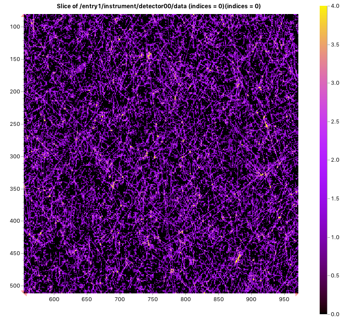
You may find this hard to imagine, but in the MAUS (our instrument), cosmic radiation is the main contributor to our detection limit, it is the noise floor which we are bound to when we are measuring freestanding samples at medium- to high Q values (see below). It is considerable enough that it adds on average about 10 counts per second when considering the entire detector surface (Figure 1). These tend to come in streaks, and with our detector lacking the ability to filter out high energy counts, these streaks add a count in every pixel it passes through.

This cosmic background for us is why we typically cannot see previously hidden information after measuring for 1h than for a 10 minute measurement. Any information we see in 10 minutes we can improve with longer measurements for better statistics. However, the balance of signal to background prevents us from uncovering more by measuring longer. In other words, we can make an ok measurement better by measuring longer, but we cannot affect our detectability by this method.

Interestingly, cosmic radiation doesn’t affect beamlines much, due to the much shorter measurement times involved. As they do not measure over several hours, the contribution of the cosmic rays is limited.

How can I determine this beforehand?

If you know enough about the system you want to investigate, and if you characterized your scattering instrument sufficiently well, you should be able to estimate directly on how visible your analyte signal will be. To do this, you can prepare a graph showing the background of your instrument for a particular sample container, where the data has not had the darkcurrent removed, without a background subtraction, and where the signal has been normalized to a nominal sample thickness (of, for example, 1 mm).

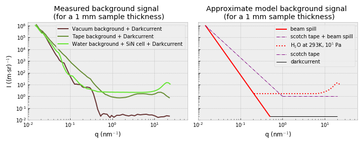
When we do this for the MAUS (Figure 2), we can directly identify what the main contributors are, and what we have to exceed. Let’s start by looking at the background signal we measure for the vacuum chamber itself, which would be a background for any freestanding samples.

This background is dominated by the beam spill from imperfect collimation at low angles, and the cosmic radiation background at wider angles. This means, practically, that your sample would need to scatter at least at the smallest Q for us to be able to reliably detect it. At angles beyond Q=1 , these samples should only scatter a bit more than the cosmic background radiation levels.

There are two ways of improving this detection limit at higher Q values. One option is to switch to a detector that can more efficiently reject the cosmic background radiation, thereby reducing its level. The second option is to use a brighter source. As the signals here are normalized by the incident flux, the relative contribution of the cosmic background radiation will reduce. The beam spill contribution, however, will just scale proportionally to your incident flux…

When measuring powders, we have to exceed the signal of the tape as shown above, which scatters more than water in its SiN low-noise cell at low angles, but less than water at higher angles. The Scotch® Magic Tape, while one of the lowest-scattering tapes on the market, has a non-negligible scattering contribution at both low- and wide angles.

Lastly, when measuring samples dispersed in water, the analyte needs to add significantly compared to the beam spill at low angles, but at higher angles you will be limited by the dispersant signal, which is far from negligible. If you have a weakly scattering sample, nothing will help you here (at high Q), unless you can do an extremely high accuracy background subtraction.

Extremely high accuracy background subtractions?

So how would you do an extremely high accuracy background subtraction? With excellent metadata, for starters. Roughly speaking, the background subtraction process can be written as , with the subscript “a” for the analyte, “ab” for analyte with background, and “b” for background (For a full description of the modular data correction procedure, please see Pauw et al., 2017).

If is only very slightly different from , not only do you need to have these scattering intensities to a very high precision, but also the values for time, transmission and flux need to be extremely precise. Any inaccuracy in these values will directly affect the subtraction by a multiple of their inaccuracy. Therefore, if you want to detect analyte signals which are of a magnitude of only 1% of the background signal, your total of six time, flux and transmission values need to be at least accurate to 99.9% (i.e. have an uncertainty smaller than 0.1%, for their fluctuation to not affect the background subtraction all too much.

At Nigel Kirby’s beamline, the accuracy in determination of their metadata, as well as the accuracy with which they determine their scattering and background signals, means they are able to identify analyte signals up to a whopping 3.5 orders of magnitude below that of their dispersant. This is a goal that, I suspect, the MAUS will never achieve.

Instrumental changes

For us, one change would be to improve the collimation of the MAUS to reduce the parasitic scattering, but which would likely also severely reduce the usable flux. Unfortunately, there isn’t a lot of space to add extra collimation, the only option would be to add another pinhole or set of slits to the vacuum sample chamber itself, directly before the sample. Then again, with the source divergence of these laboratory sources being what they are, better collimation will not get you much lower in Q. Instead, alternative methods such as Bonse-Hart’s channel-cut crystals should be considered for measuring the very low-Q region.

For synchrotrons, however, it is definitely worth fine-tuning the collimation and background to minimize their impact on the measured scattering signal and improve their detection limits, and to ensure that the metadata is as accurate as can be. This would have the biggest effect on (materials science) samples that do not rely on the analyte being suspended in water or similar solvents. For such freestanding samples, the sky is the limit.

Putting it all together:

Contributions:

So, in summary, the factors affecting the detectability of your analyte include:

1. Scattering contrast of the analyte vs. its dispersant
2. Concentration of the analyte
3. Instrumental background
4. Container background
5. Dispersant background
6. Cosmic background
7. Quality of your metadata (flux, transmission, time)

What can we affect, and what can’t be affected:

Some of these things we can improve to get a better grip on detectability:

1. The scattering contrast can be improved by changing the dispersant (as long as the dispersant is not an integral part of the sample, like it is in composites or porous materials)
2. The concentration may be adjustable, although attention should be put on making sure this does not affect the analyte.
3. The instrumental background may have a lot of room for improvement, depending on the instrument design. Improvements in collimation, reduction of beam divergence and minimizing unnecessary windows in the beam will help. Increases in flux can reduce some background contributors (see #6), but may come at the cost of beam stability.
4. The container background may be improved by choosing low-scattering materials such as Scotch magic tape for solids, or SiN windows for liquids.
5. The dispersant background cannot be significantly altered, unless the dispersant is changed altogether. Cooling down the dispersant can reduce its scattering a tiny bit, but for water is countered by the reduction in density. Cooling might also negatively affect your analyte’s ability to stay dispersed.
6. While the cosmic background cannot be affected, if the incident flux is higher, collection times can be shortened. Secondly, there are detectors becoming available that can filter out the high-energy contamination, and thereby reduce the detection of the cosmic rays
7. With improved flux-, transmission and time values you are able to do more careful background subtractions. This will help you to some degree, although avoiding the background in the first place will give you much more benefit for your effort.

What can you do right away?

I highly recommend you characterizing the background level for your instruments, so you can get a good grip of where your backgrounds come from, and what you might be able to do to improve them. Also find out with what accuracy you can determine your metadata, as these directly affect your ability to subtract the background correctly.

Additionally, get familiar (if you aren’t already) with simulating data in absolute units. This is something you can do quite easily using SasView, where the “scale” factor is the volume fraction of your analyte (for many models) once you have set the scattering length densities correct. If there’s interest, I’ll write a short blog post on this later.

Once you’ve done those two, you can now find out of that sample of exotic particles suspended in a slice of soap can be measured on your instrument, before you spend your time, energy, and CO2 (equivalent) on getting that data in real life.

Thanks to Glen Smales, Tim Snow and Andy Smith for their contributions to this story.

---

Dreiss-2006: On the Absolute Calibration of Bench-Top Small-Angle X-Ray Scattering Instruments: A Comparison of Different Standard Methods, doi: 10.1107/S0021889805033091

Kirby-2013: Kirby, N.M., Mudie, S.T., Hawley, A.M., Cookson, D.J., Mertens, H.D.T., Cowieson, N. and Samardzic‐Boban, V. (2013), A low‐background‐intensity focusing small‐angle X‐ray scattering undulator beamline. J. Appl. Cryst., 46: 1670-1680. doi:10.1107/S002188981302774X

Pauw-2017: B. R. Pauw, A. J. Smith, T. Snow, N. J. Terrill, A. F. Thünemann, The modular SAXS data correction sequence for solids and dispersions, Journal of Applied Crystallography, 50: 1800–1811, DOI: 10.1107/S1600576717015096