

We have worked on composites before, but never like this. These are the preliminary results from a series of experiments on nanoparticle-polymer composites, which have some really interesting features and might benefit from novel approaches to analysis..
A series of composites
These composites are being developed by Dr. Johanna Sänger, at my request she prepared a series of composites with increasing amount of crystalline nanoparticles (the publication on this is in preparation, which will explain the what and why). We tried – as best we could – to create a concentration series following the Renard Preferred number series (cemented in the international standard ISO 3), as it looks really good on a logarithmic scale amongst other benefits.
X-ray scattering data
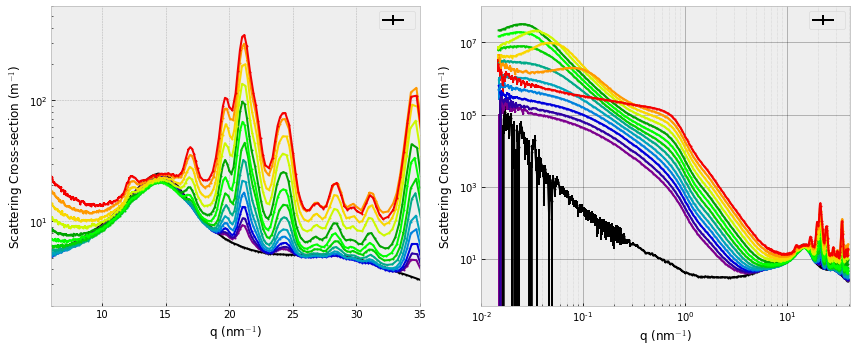
Once processed, the data actually looks aesthetically pleasing (Figure 1), the XRD region shows a nice increase in the crystalline content, and the small-angle region shows a steady increase of nanomaterial. The data here did not have the matrix phase subtracted, although that might improve the analysis. In the small-angle region of interest, the matrix scatters a few orders of magnitude lower than the sample, and so is not expected to affect the SAS analysis considerably.
One additional feature that caught our attention was the appearance of a structure factor peak at the higher concentrations. This appears first at low Q, then shifts to higher Q as the concentration increases. The increasing concentration dictates a shorter interparticle distance, effecting the aforementioned shift of the interparticle interference peak in the scattering patterns.
Wide-angle (crystalline volume fraction) analysis
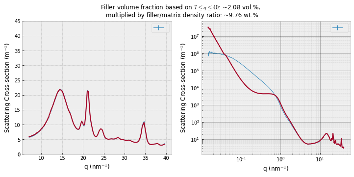
Given that these scattering patterns are so nice, they invite a thorough analysis. Firstly, we can use a method we used in the past (e.g. here) to determine the amount of crystalline material in these composites from the (absolute intensity) wide-angle crystalline signal of the mixtures compared to the pure polymer and pure nanoparticle powder. This is shown for example in Figure 2, and seems (in our experience) to give good results for materials that don’t physically change when embedded.
Small-angle (nanoparticle dimension) analysis
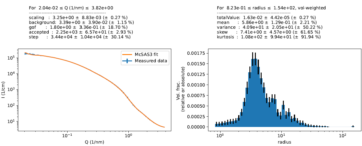
Next up is the small-angle scattering region. For the lower concentrations, it is perfectly fine to use a normal McSAS run with spheres (or now McSAS3 for those not afraid of a command-line interface). The assumption of the spherical nature of these scatterers was supported by TEM imagery. We get a distribution out that looks pretty reasonable (Figure 3)…
Small-angle analysis of high-concentration data
For the higher concentrations, we want to check that the size distribution is not affected by the higher concentrations. It could be, for example, that a particular size in this distribution is more prone to agglomeration than others. That, of course, means introducing a structure factor in McSAS3 (I did try resolving this with a classical fit in SasView with a sphere formfactor, an analytical size distribution and a volume fraction, but it didn’t work anywhere near as good as McSAS3). While the inclusion of SasModels in McSAS3 has its drawbacks, the benefits are that it comes with fancy structure factors. So after a little adaptation of the code (because it works slightly differently with structure factors), I got the hard-sphere structure factor with beta-approximation working for sphere models.
That leaves just one problem: this needs the input of a local volume fraction. If I use the actual volume fraction, it doesn’t always get me a nice fit. This is likely related to either 1) the limitations of the structure factor approximation, or 2) slightly imperfect dispersion of the nanoparticles in the matrix, leading to locally higher concentrations of nanoparticles. So how to we test for option 2? I don’t have the option of a least-squares fit of this parameter before the optimization is finished, and applying a post-hoc structure factor to the above distribution isn’t as pretty as it could be (limitations rearing their ugly head again).
Applying the brute-force local volume fraction optimization to all samples
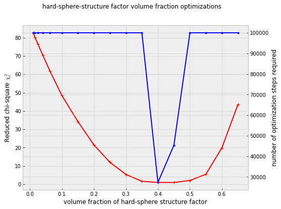
My attempt at resolving this was to start a series of McSAS3 optimizations with stepwise increasing (local) structure factor volume fractions. As you see, my solution to many problems is to throw even more computing power at it. The initial test on one of the higher-concentration samples looks promising, which should have a volume fraction of 20%, but fits best with a local volume fraction closer to 40%. Time to try that on the remaining samples.
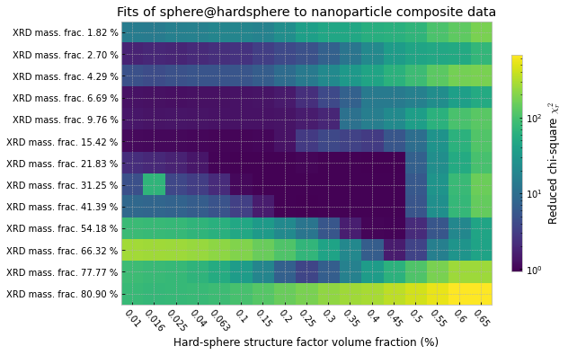
After a full week of calculating on 30 cores, this has now completed. The results in Figure 5 show that it is maybe a reasonable approach, and seems to give optimal points (lowest chi-squares) for volume fractions that aren’t all too crazy. There are outliers, and it seems to break down for the highest concentrations for some reason (maybe I’m outside the region of applicability for this structure factor approximation).
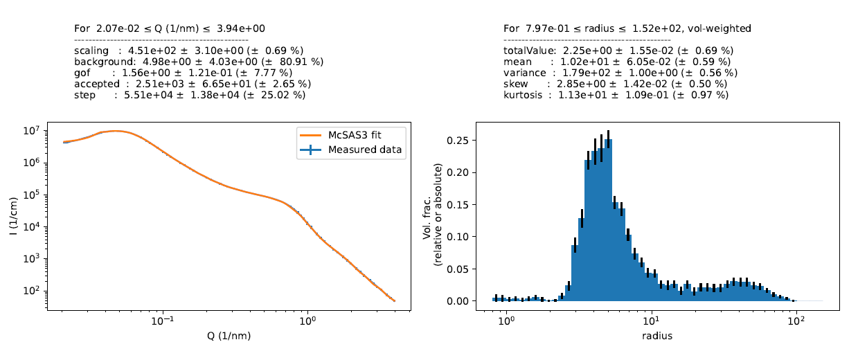
It seems like the sample with a 66% mass fraction was the last that showed a reasonable result. We can check to see what that size distribution looks like and if it is like the one we saw before. A first look in Figure 6 shows that we do have a different resultant size distribution, with a much larger mean particle size and what looks like a population of larger particles. Whether or not this is a realistic representation of reality will need to be verified with complementary techniques.
To be continued…
This has been the work over many months of preparation, measurement, processing, analysis and interpretation, and we’re not done yet. There are a few series of these composites prepared, and they each need this kind of analysis. I’m not 100% confident yet that the brute-force approach is able to extract realistic information, but so far it has not delivered unphysical results or results outside of expected ranges (apart for the highest concentrations).
Leave a Reply