Skip! A way to ignore diffraction peaks in a McSAS3 fit

Over the years, we’ve had more than a few complex samples which showed diffraction peaks from regular structures intermixed in the small-angle scattering signal from the irregular scatterers. This has been a problem for McSAS, which is why we (or rather, my colleague Glen Smales) then would resort to tedious modelling of the complete pattern using SasFit or SasView, diffraction peaks and all. Now we have a pragmatic solution that at least will help your initial fits: you can omit data ranges from a McSAS analysis, allowing you to use the full range unencumbered by those pesky peaks…

While diffraction peaks contain important information on a part of the morphology of your sample, their origins may lie in structural features that are disjointed from the structures effecting the scattering signal we want to analyse with McSAS. For example, we may have scattering from small, disordered clusters, but have a diffraction signal from a separate crystalline phase interfering. In that case, we want to analyse the one signal without interference of the diffraction peaks.

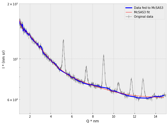
Case in point: some metal-organic framework data from my colleague shows the MOF diffraction peaks in a region where small disordered clusters are also visible. As these MOF peaks are quite sharp and do not move, we can cut their data ranges away to be left with the surrounding intensity.

This is not the best way of dealing with these: in the most ideal case, we would include peak shapes and analyses in the description of the total intensity, and take them into account this way. However, to make this a universally applicable option in McSAS3, for example, would add an enormous amount of complexity, which would also slow the process down considerably (as each peak’s parameters would need to be optimized in the least-squares step that now just optimizes the scaling and background factor). That would add a lot of instabilities into the system too.

The more pragmatic “ignore these data ranges”-option was easier to implement, though, and it might help you too. These ranges can be set up using the “omitQRanges” keyword in the YAML configuration file for the data read-in. For example:

--- # configuration used to read nexus files into McSAS3. this is assumed to be a 1D file in nexus
# Note that the units are assumed to be 1/(m sr) for I and 1/nm for Q
# if necessary, the paths to the datasets can be indicated. 
nbins: 100
dataRange:
  - 1.0 # minimum
  - 15 # maximum for this dataset. Positive infinity starts with a dot. negative infinity is -.inf
pathDict: # optional, if not provided will follow the "default" attributes in the nexus file
  Q: '/entry/result/Q'
  I: '/entry/result/I'
  ISigma: '/entry/result/ISigma'
omitQRanges:
  - [4.9, 5.5]
  - [7.1, 7.6]
  - [8.8, 9.4]
  - [10.2, 10.8]
  - [11.4, 12.0]
  - [12.5, 13.1]

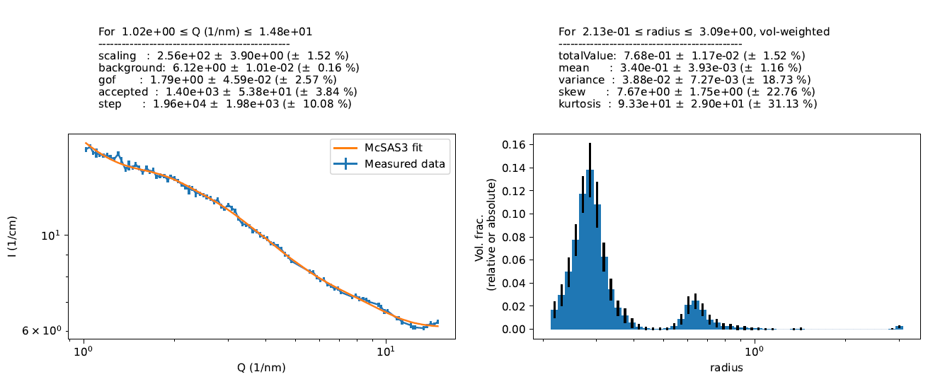
This then lets us skip the regions as shown above, and we can do our McSAS3 fit to get the population information out as needed (note, volume fraction absolute scaling is still incorrect here). All in all, not bad for a few days’ programming. The McSAS3 codebase (still under development) can be obtained here.