Those of you who have been around this blog a while, know that we have also been dabbling in laboratory automation (see, for example, this post).
Over the last year or so, led by my former colleague Dr. Glen Smales, we used RoWaN to synthesise over 1200 Zeolitic imidazolate frameworks-8 (ZIF-8) metal-organic framework samples spread over 20 series, while systematically varying many synthesis parameters. Changing seemingly innocuous aspects appears to have a strong impact on the final particle size (distribution), so a correct logging of the metadata is essential for correlating synthesis parameters with morphology.
We have presented this work several times already in various presentations (one of which should go online soon) and large manuscripts are in the works with the full story. Given the scope of this investigation, preparing these manuscripts eats up a lot of time. Today, I would like to focus on how we structured the synthesis metadata that was collected for every sample.
Since small synthesis details might correlate with the resultant particle morphology, we went overboard with the metadata collection. Everything we could think of and get access to, was recorded and integrated in the final structure. This includes such things as bottle opening dates and the humidity in the laboratory. This “everything and the kitchen sink”-approach has saved our bacon a few times in the past when debugging MOUSE measurement issues, and will probably not be out of place here either.
Data Sources
The data sources here were varied, we take what we can get, how we can get it: some data comes from the log of RoWaN itself, which can store such things as EPICS messages as well as step messages (e.g. “Start injection of solution 1”, and “Stop injection of solution 1”) in a long CSV file. Some manual steps were recorded manually using predefined messages in predefined cells in the Jupyter notebook. Some instrument readings (density meter reading for example for the stock solutions) is read manually and added to the log by hand.

Data on the starting compounds / chemicals and equipment comes from a master Excel file that contains this information in a structured manner across several sheets. We use Excel because it is a pragmatic user-entry system that does not require any training and whose output can be read with Python. It has severe restrictions, though, that would preclude its use in larger projects and an easily-configurable web form solution is still sought (hook me up when you know of one that can take external yaml or json files specifying configuration of pages, parameters, data types and limits).
Translation, translation, translation
During my last presentation at FAIRmat, there was a good set of questions from the audience about if we can (or should) dictate what, and in what format this metadata should be recorded. At the moment, I would shy away from such efforts. On the one hand, it is impossible to predict what you will need in the end, so I would advise to record everything. On the other hand, any additional workload on an already overloaded workforce is bound to be hated, ignored or forgotten, so chances are that you will not get it as you intended anyway.
Better to encourage recording whatever low-hanging fruit are reachable as automated as possible. You can hook up your heating/stirring plates, syringe injectors, thermometers etcetera to a laboratory network and, with a little effort, continuously read out what they do in whatever format they do it in. Make it as simple as possible to record this, lower the threshold for such documentation, and only require manual documentation if it can somehow absolutely not be avoided. You will get a collection of files and will need to translate that into useful information probably together with some custom knowledge and lots of time stamps. This, in my eyes is unavoidable, although the eventual introduction of a message broker would help greatly. As it is now, we spend a significant portion of our code translating between what we get and what we need, adding some domain knowledge into the code.
We made a piece of software called DACHS that does this. Most of this code defines generic data classes for the various objects and information entries that we want. Values and units, where possible, get translated into unit-aware quantities with Pint, which makes it extremely easy to do unit-aware calculations with, say, moles, grams and millilitres and combinations thereof. The value of this ability cannot be overstated.
One non-generic segment of the code, however, is focused on applying those models to our specific data sources, and to subsequently structure these into a specific tree for this experiment. So what does this tree look like?
The base tree
We decided to split our base tree into three sections: “Equipment”, “Chemicals”, and “Synthesis”, which contain what they say on the tin (Figure 1).
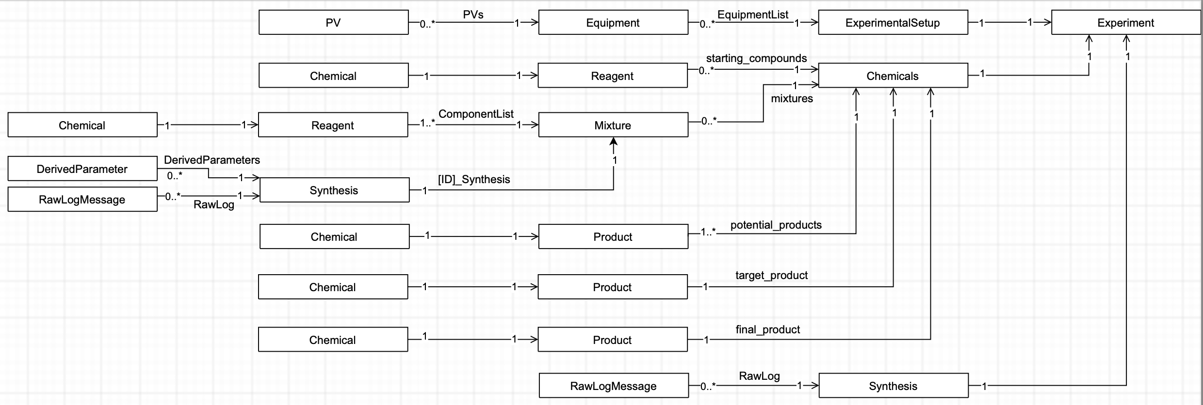
The Equipment section contains a list of the equipment used for that particular experiment (this can vary between experiment series). Equipment includes such things as stirrer bars, Falcon tubes and tubing, as this might correlate to the result. Each equipment has detailed information including which PVs, or “Process Variables” they control. These PVs can contain linear calibration information, i.e. split over a calibration offset 


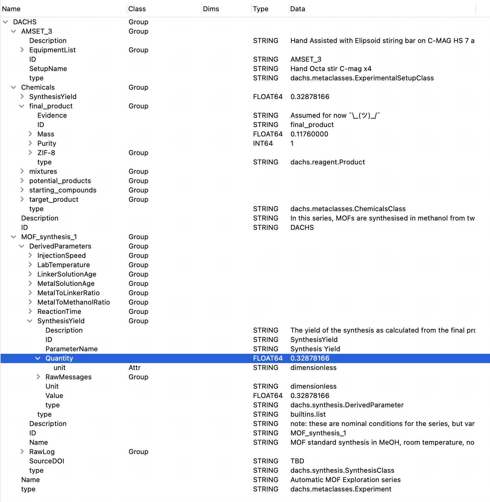
The Chemicals section is split into several parts, beginning with the starting compounds. These contain the base reagents as found in the jars of the suppliers. Each reagent has information such as supplier, CAS number and lot number, as well as jar opening date (if known). It also contains information on the chemical in the reagent, with chemical formula, molar mass, density and space group (if known). See Figure 2 for a bit more information on how deep we go with this.
Limitations
Here, it perhaps behooves to highlight that the solution here is a pragmatic proof-of-principle solution mostly resulting from the effort of less than a handful of people. There are limitations aplenty, for example, there is probably a spate of parameters we are not – but should be – logging.
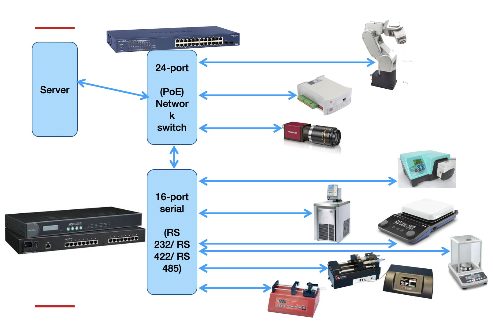
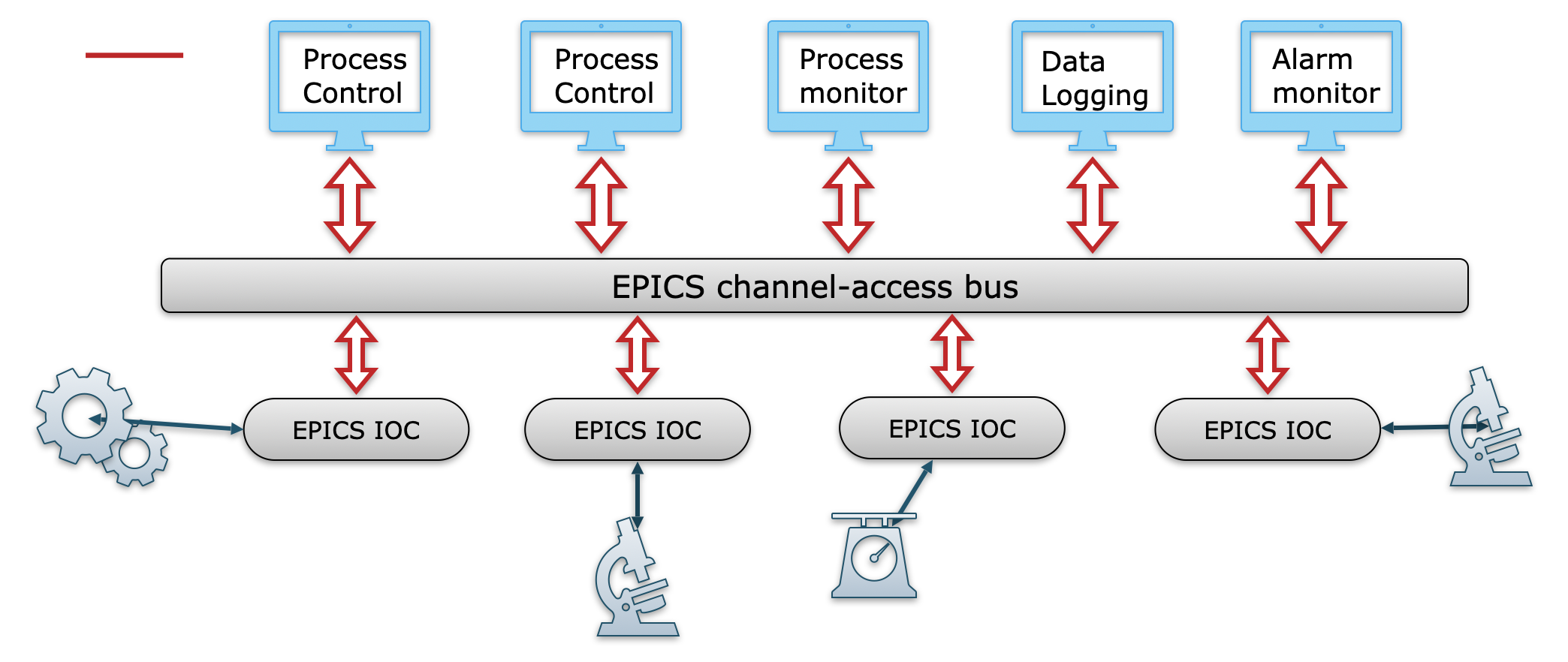
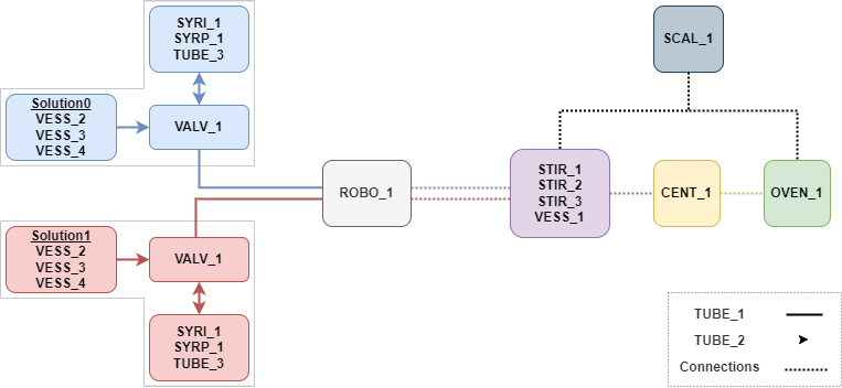
One thing I could not figure out how to implement easily is equipment interconnectivity. Equipment is connected on several levels: an electrical level (Figure 3), a virtual level (figure 4), and a synthesis-side physical level (tubing etc, Figure 5). So this information is missing from the structure and only exists as vector graphics hand-drawn using the draw.io software. I’m sure there is a better way.
Then there is the matter of uncertainties. For someone who keeps hammering on about the value of uncertainties and even splitting them up into different classes of uncertainties (“absolute” and “relative”, see the Everything SAXS paper), it is quite hypocritical of me to not have added them here. I decided against it in the end as none of the uncertainty estimates I could come up with were grounded in any sort of realism, i.e. all of them would be guesstimated and therefore would not have any weight to them. Maybe at a later stage it can be improved.
Also, I had initially provisioned for a more defined synthesis step (called SynthesisStep), which theoretically should allow classifying each synthesis step. This, in turn, should form a good step (ha) towards automatically recreating a synthesis using another robot.
in the end I did not include this as the more I worked with it, the more I realised that most of its purpose is already performed by RawLogMessage. And any universality with other robot systems is moot if I don’t tailor it to use the confines of other robot system concepts.
Here, too, translation will be essential to turn the information contained in these synthesis logs into a synthesis protocol for other robots to use.
So where to go from here?
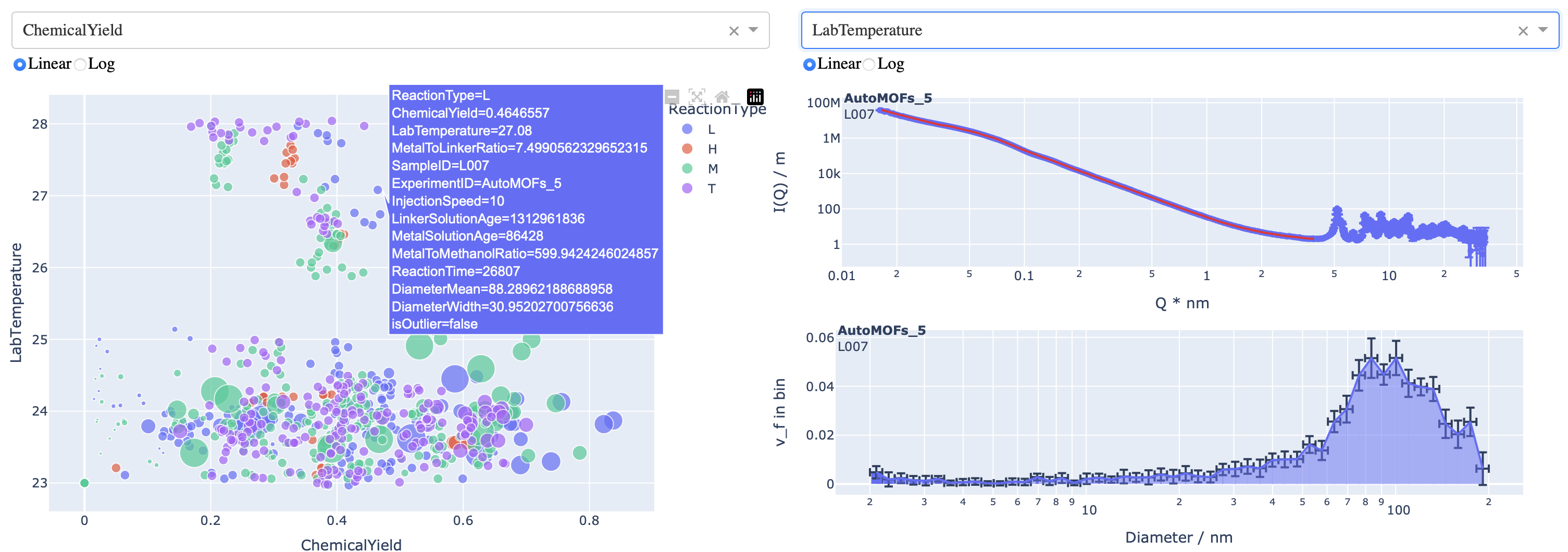
With the information encapsulated in the synthesis files, we can now start exploring. I’ve built a simple dashboard using Dash and Plotly that allows one to plot parameters against another. Additionally, for samples that have been measured already, the scattering pattern and size distribution can be shown too (indeed, the resultant size parameters are plottable too). This allows a bit more information to be gleaned, but the two-dimensional nature of the plotting isn’t really enough to extricate the necessary interparameter correlations. That will require a bit more effort.
Nevertheless, it’s pretty, and that will suffice for now! (see Figure 6)