

By the way, my topical review paper on SAXS data collection and correction has been published and is available open access here!
Recently, some good colleagues (who are not familiar with scattering) have started asking questions on how to go about fitting a scattering pattern. This was a very good opportunity to think about the process from a layman perspective. How do we get from scattering pattern to morphological information in a straightforward way?
For me, this typically takes about three steps: 1) the initial look, 2) some simple fits and 3) the final fit. There is a possible fourth step: advanced fits, but this is not a necessity in some cases. This post will focus on the first step: the initial look.
So imagine you have collected a scattering pattern and subjected it to the applicable corrections to get a background-subtracted, corrected scattering pattern. This sets the stage for step 1. In step 1, we check if there is any suitable information in the scattering pattern at all, and we collect information from other techniques.
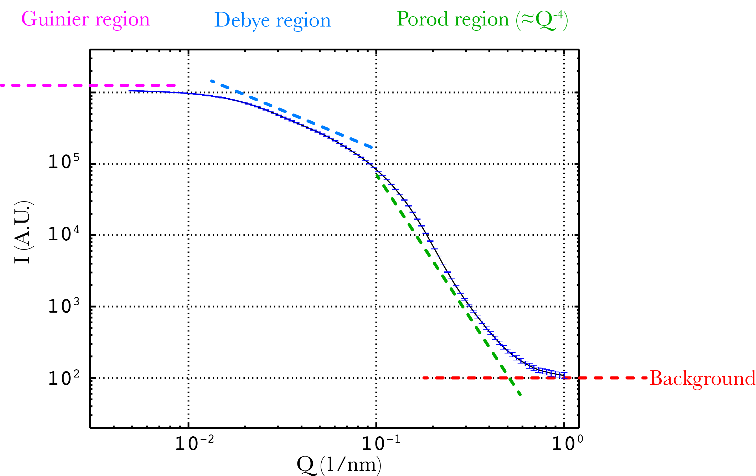
What I’d do is to plot the data on a double-logarithmic plot, in intensity versus scattering vector: 

The constant background contribution can arise from a plethora of causes. It can come from very small-scale inhomogeneities in one or both of the phases in your sample, or remains from insufficient background subtraction or insufficient correction for detector darkcurrent levels [1,2]. There is a modicum of information in the background level, but usually it is partially or wholly artificial.
The Porod region is another region of limited use. The scattering intensity in this region should be proportional to a 
Porod slopes smaller than
At q-values lower than the Porod slope, there can be a region which contains the most information in the scattering pattern which I shall call the Debye region (after the early description of this region by Debye, Büche, Anderson and Brumberger [6,7]). This region typically has a slope between 

Some say that a particular slope identifies the shape of the scattering entities (discs, cylinders or spheres), but this is not completely unambiguous. As will be shown later, the scattering pattern from polydisperse cylinders can be perfectly described using spheres as well (though perhaps the reverse does not hold, I did not test that yet…). All that can be said, then, is that this region is the one carrying the information.
Before that Debye region lies the Guinier region: a flat region independent of q. This contains information on the volume-square weighted size of the scatterers, and also can be used to find the total volume fraction of scatterers in the sample. As it typically lies at very low q values (and so very close to the beamstop), it is also most easily affected by parasitic scattering and other unrelated scattering effects. In short: This region has some information, but is prone to fouling.
Figure 1 shows the best case scenario for data: that in which all regions are clearly visible and distinct from one another. I will provide a few more examples to indicate some alternatives you might find in your scattering patterns.
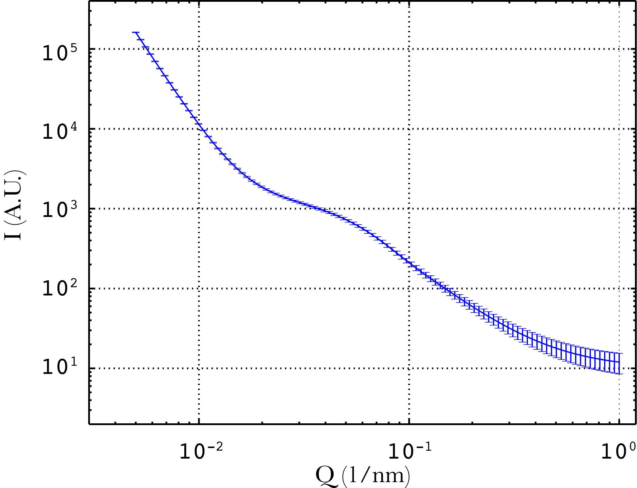
Figure 2 shows another situation where there is a certain amount and distribution of discs (the hump in the middle), and a background contribution. I also simulated the presence of some larger structures (i.e. aggregates or simply large scattering objects), of which only the
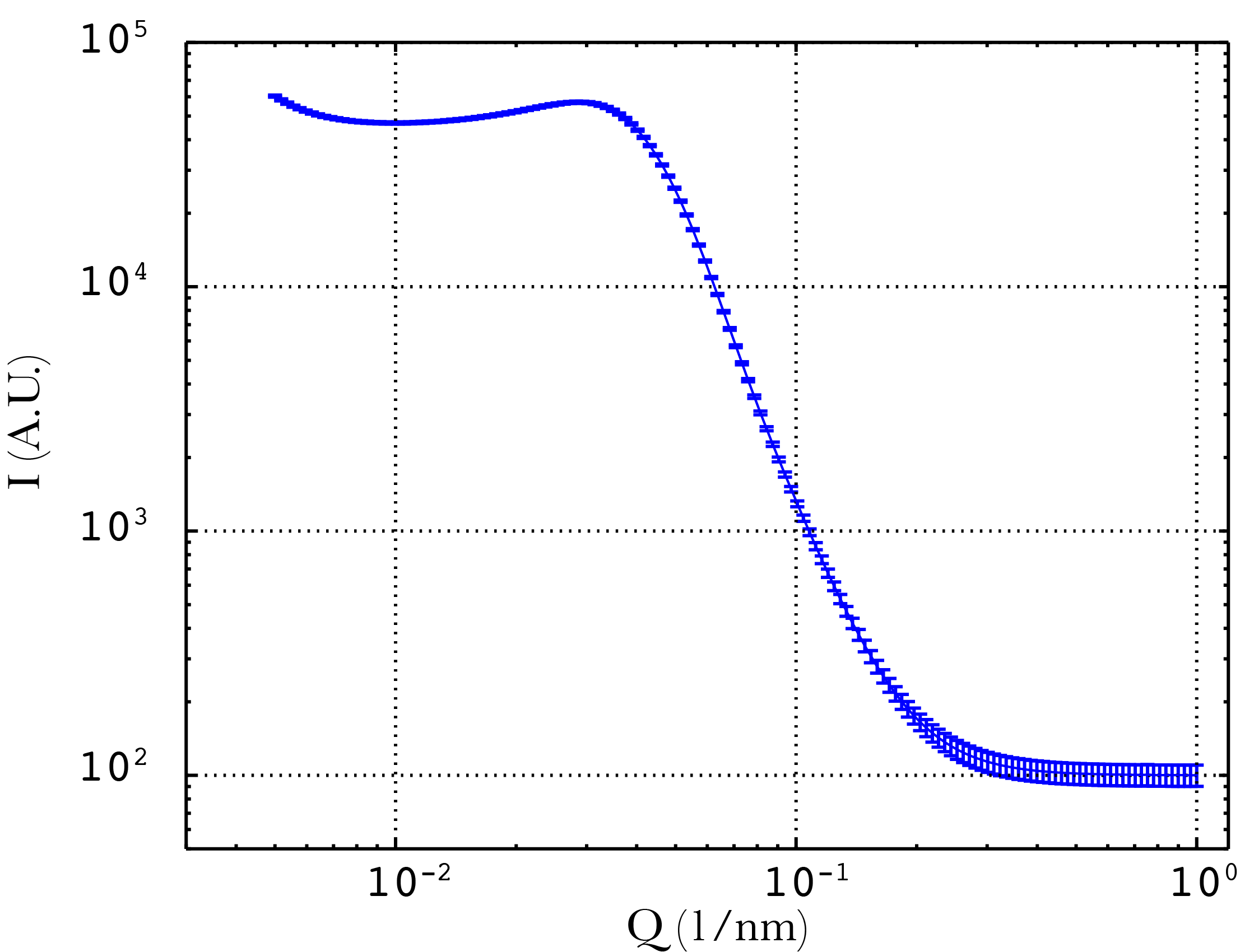
Figure 3 shows an interesting case of scatterers (spheres in this case) which are quite densely packed. This dense packing causes inter particle interference which shows up as a depression in the scattering pattern. It may not necessarily be as clear as this, and its visibility can reduce due to a plethora of effects (polydispersity, background, etc). Structure factors can be a pain in the ass to fit. Diluting the sample to remove this effect is recommended if possible.
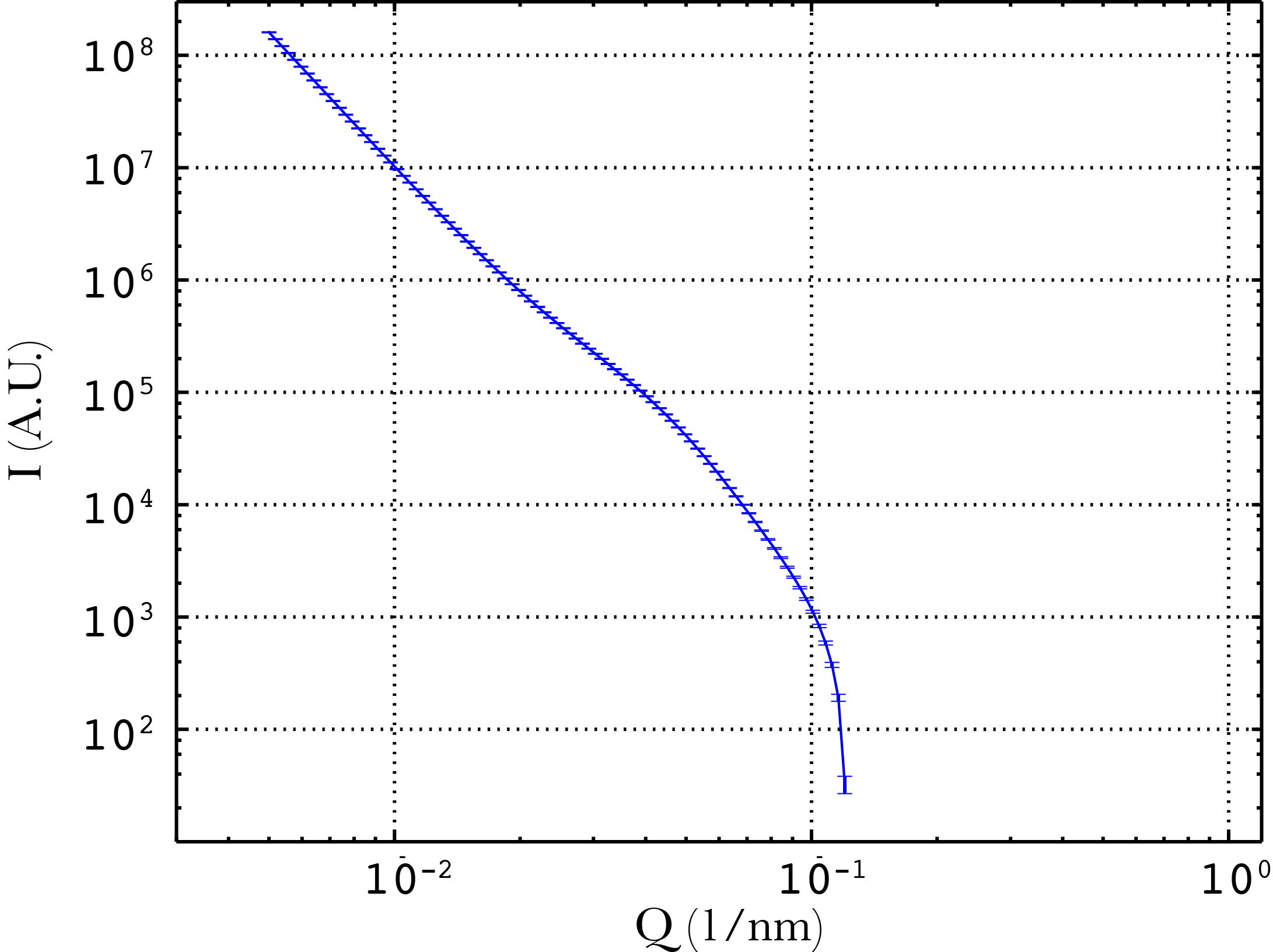
A common problem in data correction is that of oversubtraction of the background measurement (because people tend not to correct for transmission). Fortunately, it is easy to recognise this mistake, as shown in Figure 4: there is a marked drop to negative values of the scattering signal at higher q-values.
The simulations shown here are made using SASfit by Joachim Kohlbrecher and Ingo Bressler. I highly recommend downloading that software, to learn how to use it and to simulate a few scattering patterns to get a feel for what small-angle scattering can look like. Another good package is the Irena package by Jan Ilavsky for Igor Pro.
Next up in this series: part 2: basic fitting.
[1] W. Ruland. Small-angle scattering of two-phase systems: determination and significance of systematic deviations from Porod’s law. J. Appl. Cryst., 4:70–73, 1971.
[2] J. T. Koberstein, B. Morra, and R. S. Stein. The determination of diffuse boundary thicknesses of polymers by small-angle x-ray scattering. J. Appl. Cryst., 13:34–45, 1980.
[3] R. Sobry, J. Ledent, and F. Fontaine. Application of an extended porod law to the study of the ionic aggregates in telechelic ionomers. J. Appl. Cryst., 24:516–525, 1991.
[4] J. Teixeira. Small-angle scattering by fractal systems. J. Appl. Cryst., 21:781–785, 1988.
[5] G. Beaucage. Small-angle scattering from polymeric mass fractals of arbitrary mass-fractal dimension. J. Appl. Cryst., 29:134–146, Jan 1996.
[6] P. Debye and A. M. Bueche. Scattering by an inhomogeneous solid. J. Appl. Phys., 20:518–525, 1949.
[7] P. Debye, H. R. J. Anderson, and H. Brumberger. Scattering by an inhomogeneous solid. ii. the correlation function and its application. Journal of Applied Physics, 28:679–683, 1957.
Nice article, Brian. I wish I could do all of my fitting in those 3 steps!