USAXS in the MOUSE: proof-of-principle results

Earlier this year, we published our work on the possibility to extend a synchrotron beamline with an inexpensive Ultra-SAXS module. The intention was that this module could be dropped into a good laboratory SAXS instrument as well, such as our MOUSE, but this turned out to require a few more modifications than we were ready for at the time. These, however, have been addressed, and so a few weeks ago, we were able to run the first few trial measurements with a USAXS module in the MOUSE. Here are the initial results…

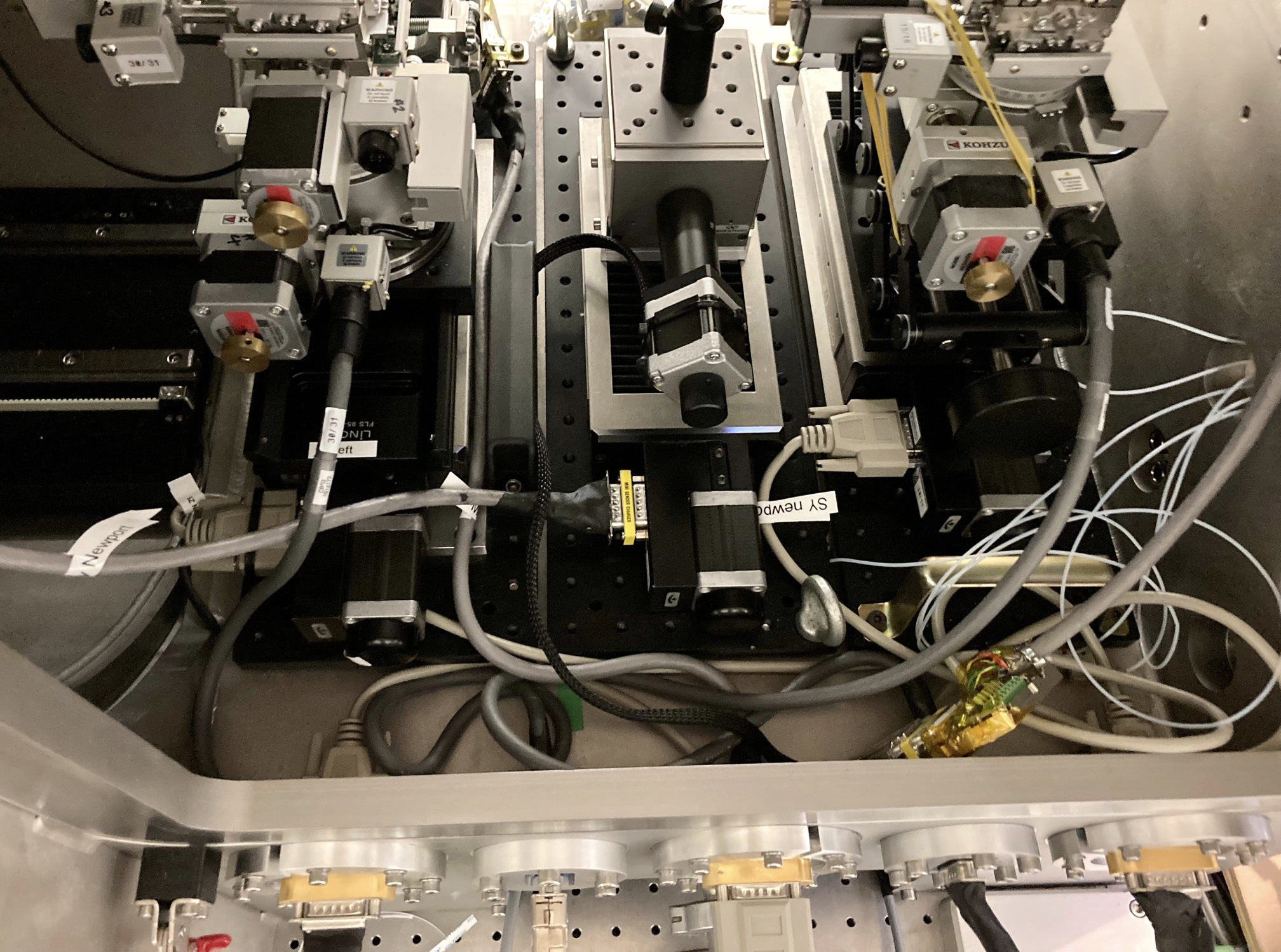
Firstly, the stages needed to be rearranged so that the rotation axis was more centered. This meant shortening the rotation arms and rearranging the components so that they would fit without interference in the MOUSE vacuum chamber. This was more involved than I had initially imagined, as the USAXS has one high-precision motor that sticks out quite a bit, in addition to relatively bulky rocking stages, each of which could bump into something else in unexpected ways.

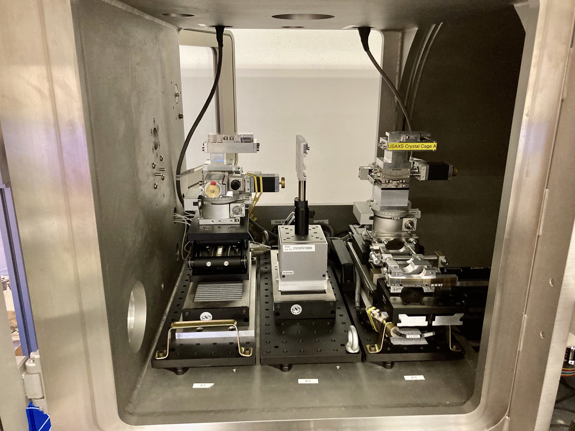
On the MOUSE side, we needed to adapt the chamber include additional vacuum feedthroughs for the 15-pin d-sub connectors that connect the total of seven motors: two motors for the upstream crystal stage, two for the sample stage, and three for the downstream crystal stage. At the same time, we needed extra motor drivers that could drive all these motors, for which we chose the very capable, yet relatively inexpensive six-axis TMCM-6210 controller/drivers. These, however, also needed to be supported in the SPEC software, which took some more effort by the main SPEC developer.

We then took a day every week, to step-by-step introduce the components in the MOUSE instrument and try connecting and aligning each of them in turn. First the upstream stage, then the downstream stage, then the new heavy-load sample stage (needed due to possible collision risk with the normal sample stage), and finally all three. At each step, we fought with cabling locations, connector wiring, motor calibrations and limit switch behavior. Finally, though, it seemed like everything was working as it should. Trials in vacuum seemed to show that the non-vacuum-“compatible” items were, in fact, vacuum compatible (although we probably evaporated quite a bit of grease out of the bearings in the respective stages, which I am now replacing with high-vacuum grease where possible).

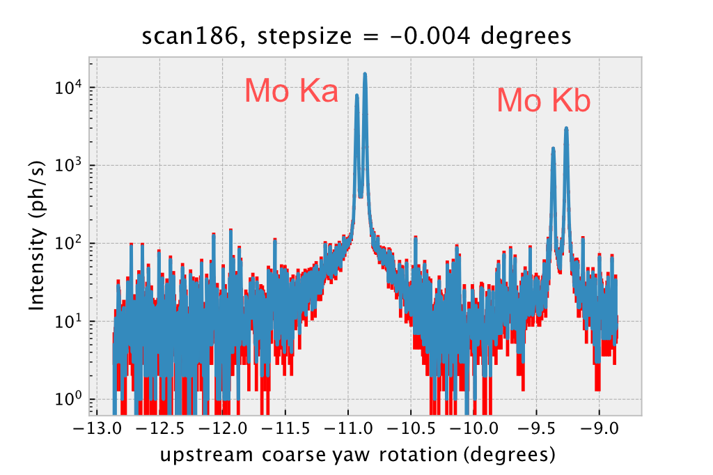
Alignment was fairly straightforward, as it turns out, we need to level the crystals in pitch and roll (we can do this by hand to 0.1 degree), find the inner edge of the channel in the crystal, and rotate to the angle for the Si220 reflection at that energy (10.7 degree in our case). We can then scan the upstream crystal and get an energy spectrum for our source for free (see Figure 4). The spectrum was a little surprising as we thought the k-beta radiation would have been filtered out by the optics, but it appears in pretty much the original strength. It could be that the optics are slightly misaligned – learned something and will find out more. The downstream crystal is a bit harder to align, because now we only have a very parallel beam with a narrow energy bandwidth, so we have to very carefully step scan not to miss the beam. However, it’s mostly where we think it should be so usually we find it on the first or second try.

Lastly, we needed a custom measurement script that could do the USAXS scan the way we imagined, yet following the methodology that we have set up around the instrument. Mimicking the settings we used for the previous synchrotron experiments, we could configure a stepped scan with enough points at the right spacing to give us a good USAXS curve, but not too many to make it impractical to measure. We now collect a detector image of the beam at each analyzer crystal rotation, so we can crop it later to maximize the signal-to-background ratio (cosmic radiation defines our background levels). The detector images can be seen in Figures 5a and 5b, without and with sample respectively.

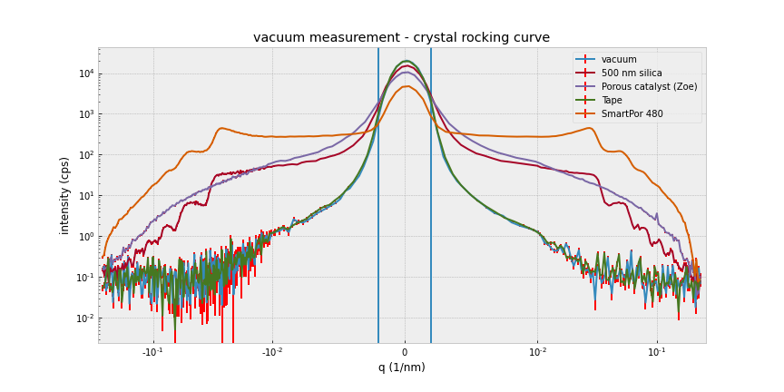
After the first scans, I processed the data in a prototype script (eventually this will be taken over by DAWN), and after some tweaking managed to get some pretty neat results for the samples we measured: vacuum, tape, 500 nm silica, an alumina membrane with 480 nm-spaced pores, and a catalyst material. Signal-to-noise seems very acceptable, and the instrument behaved reproducibly during the four days of measuring. Alignment of the crystals needs some finesse due to the angles involved, but again, it demonstrates that USAXS doesn’t require as much as we would imagine. Not even in the lab.

To conclude, here’s a quick summary and a listing of outstanding issues:

• We are working with a not so bright Molybdenum source, coupled with a 50% detector efficiency. The beam is about 750 micron in diameter, and has about 30000 counts per second in the beam at the sample. Not great, but we can expect a >7x increase once we switch to copper (the current crystals are not compatible with this)
• The stages seem to work in vacuum, bu I’ll need to take everything apart and re-grease the stages as best I can with high-vac grease, in particular the high-precision rotation bearing. The Kohzu rotations are also in need of servicing and realigning by Kohzu.
• The interferometer strip is not connected at the moment (lacking another feedthrough, and I’m not sure how well the readout module will cope with vacuum). The fine yaw rotation seems to behave well though.
• In the current measurement scheme, a sample measurement takes about 15 hours, but we are scanning quite wide, both ends, and have about 1 decade overlap with the normal MOUSE range for strongly scattering samples
• There is a lot of signal-to-noise to be gained from intelligent cropping of the 2D detector images; careful cropping will reduce the cosmic ray signals. These can also be removed by using our SDD instead of the Eiger 1. An Eiger 2 would also be able to filter out 75% of cosmic radiation, but we don’t have one at the moment.
• It takes 7 hours to set up and align the seven motors in the MOUSE, not far off of the 6h it took at I22.
• I haven’t programmed a desmearing routine yet, which we could subsequently transcode into a DAWN processing step.
• The data files need to be stored in a suitable archival structure, whilst being compatible with the DAWN processing pipeline. I’m rewriting this at the moment.
• The cables need reworking, the vacuum feedthroughs we have ‘mirror’ the pinout, and I needed to reverse this in the cables. This has led to heavy and stiff cables which are interfering with a smooth operation. I’ll rewire the motor controllers so that their outputs are mirrored instead, and we can use normal off-the-shelf cables.
• Knowing what we know now, I can simplify the design considerably making it easier to use. Stay tuned for the next iteration!